Chapter 14: GeoAI, Machine Learning, and GeoRAG Concepts

GeoAI applies artificial intelligence to spatial data and spatial problems. GeoRAG extends retrieval augmented generation by grounding language model responses in geographic context, spatial documents, maps, datasets, and location-aware retrieval.

Companion visual reference: Spatial Data Structure Visual Atlas

Learning Goals

• Explain why geospatial ML differs from ordinary tabular ML.
• Prevent spatial leakage in model training and evaluation.
• Understand spatial embeddings, Earth observation foundation models, and graph ML.
• Design GeoRAG systems that retrieve and reason over spatial context.

Theory

Spatial data violates many assumptions of ordinary machine learning. Nearby observations are often correlated. Training and test samples can leak through space. Labels may be uncertain, biased, or scale-dependent. A model can perform well in one region and fail elsewhere.

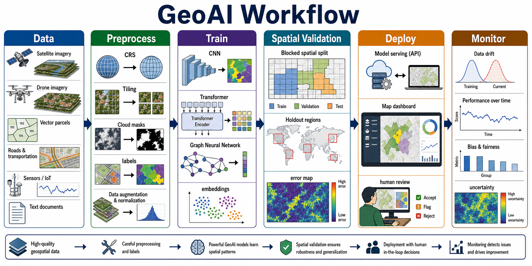
GeoAI is not one technique. It is a family of workflows that apply machine learning to spatial questions:

• Computer vision on imagery: classify land cover, segment buildings, detect roads, count trees, identify burn scars, map flood extent, or detect damaged structures.
• Raster and data-cube learning: model multiband imagery, climate grids, elevation, weather, soil, and time-series observations.
• Vector feature learning: predict parcel risk, classify road segments, identify suspicious edits, score site suitability, or estimate demand.
• Graph learning: model road networks, utility networks, river networks, transit systems, supply chains, and mobility flows.
• Spatiotemporal forecasting: predict wildfire spread, traffic congestion, crop stress, disease risk, flood depth, or demand at future times.
• Spatial embeddings: represent places, images, cells, routes, or regions as vectors that can be searched, clustered, compared, or used as model features.
• GeoRAG: retrieve spatially relevant documents, datasets, maps, and metadata so a language model can answer with place-specific evidence.

The key difference from ordinary ML is that location is not just another column. Location controls neighborhood effects, sampling bias, scale, laws, physical processes, and model validity. A model trained on coastal imagery may fail in desert cities. A crime model may learn policing patterns rather than crime. A crop model may confuse soil brightness, irrigation, crop type, and sensor season. A GeoRAG system may retrieve the wrong ordinance if it ignores jurisdiction boundaries.

GeoRAG adds another layer: retrieval must understand place, scale, geometry, time, jurisdiction, and source authority. A system answering "Can I build here?" must retrieve parcels, zoning, flood zones, policy documents, and local rules, then state uncertainty and provenance.

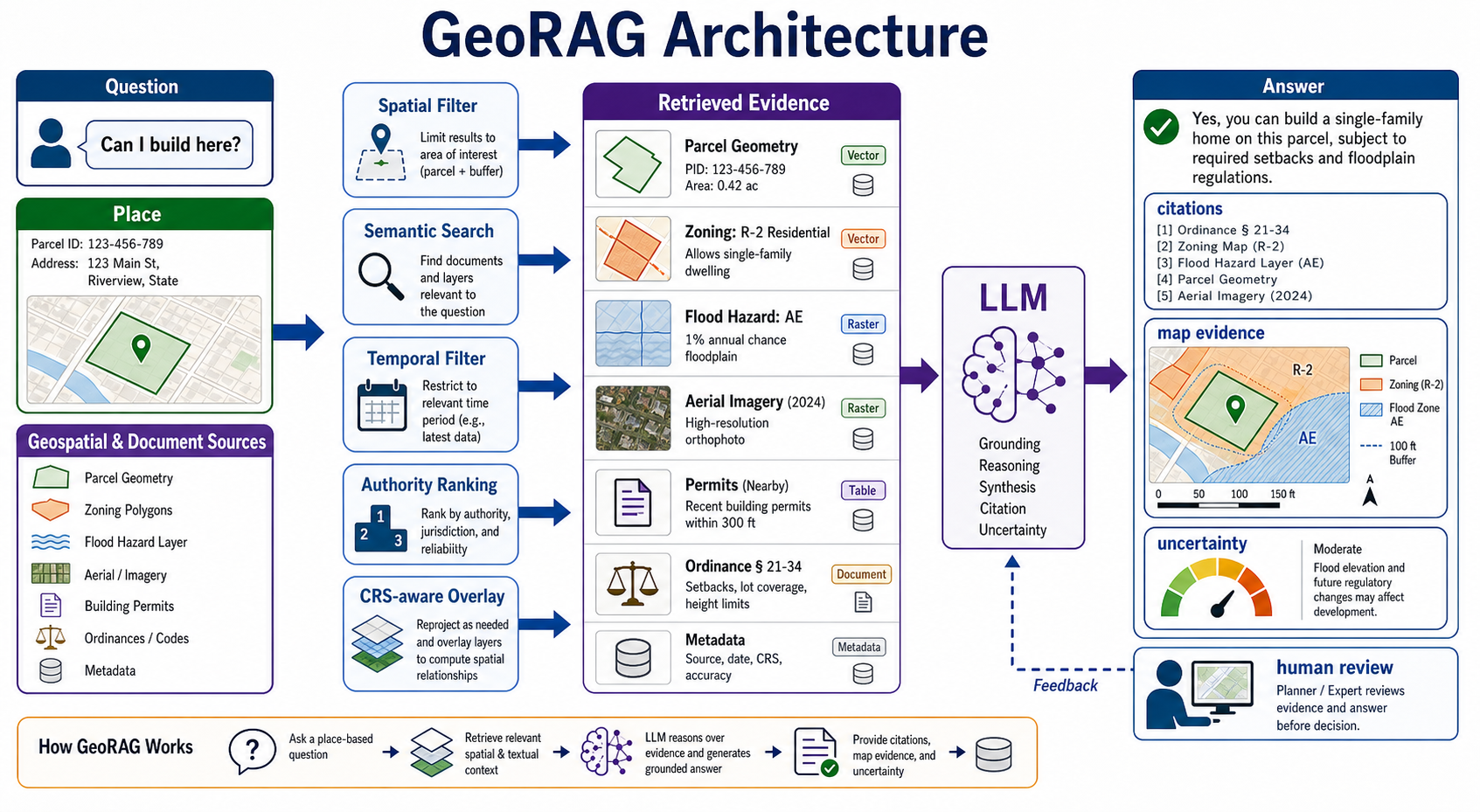
GeoRAG systems combine language retrieval with spatial operations. A good GeoRAG answer should be able to say:

• Which geometry was used as the area of interest.
• Which CRS and spatial operations were applied.
• Which documents, map layers, datasets, and metadata were retrieved.
• Which sources were authoritative for the jurisdiction and date.
• Which spatial relationships were computed, such as intersects, contains, within distance, upstream, downstream, nearest, or inside service area.
• What uncertainty remains and when a human expert should review the answer.

GeoAI Task Patterns

Task pattern	Typical inputs	Typical output	Example
Classification	Image chips, vector attributes, environmental covariates	Class label or probability	Land cover class, roof type, crop type
Semantic segmentation	Imagery, elevation, masks, labels	Pixel-level class map	Building footprint, water extent, road surface
Object detection	Imagery or video	Bounding boxes, points, counts	Vehicles, solar panels, damaged buildings
Instance segmentation	Imagery, prompts, masks	Object-specific polygons or masks	Individual tree crowns or rooftops
Regression	Raster/vector features, time series	Continuous value	Yield, flood depth, heat risk, population estimate
Forecasting	Time series, weather, mobility, sensors	Future state or trajectory	Traffic, fire spread, crop stress
Graph prediction	Network topology and attributes	Edge/node score or path behavior	Road congestion, utility outage risk
Similarity search	Embeddings for places, imagery, documents	Nearest neighbors or ranked candidates	Similar neighborhoods, image search, site analogs
GeoRAG question answering	Text, maps, geometry, metadata, embeddings	Grounded answer with citations	"Is this parcel in a floodplain?"

Foundation Models and Transfer Learning

Foundation models are increasingly important in GeoAI because labeled geospatial data is expensive. Remote sensing foundation models can learn from large collections of satellite imagery or weather data, then be fine-tuned for tasks such as flood mapping, cloud detection, land-use change, burn scar detection, crop monitoring, or disaster response. As of May 2026, NASA has reported Prithvi-based geospatial foundation model work trained on Harmonized Landsat and Sentinel-2 data and demonstrated in orbit for flood and cloud detection. Tools such as TorchGeo make it easier to build CRS-aware geospatial deep learning pipelines with samplers, datasets, transforms, and pretrained backbones.

Foundation models do not remove the need for geospatial judgment. They still need:

• sensor metadata and band definitions;
• CRS, resolution, tiling, and resampling discipline;
• cloud, shadow, nodata, and quality masks;
• labels with known provenance;
• spatially honest validation;
• uncertainty maps and human review;
• monitoring for region, season, sensor, and policy drift.

Promptable models such as Segment Anything can accelerate annotation and segmentation workflows, but the outputs still need geospatial validation. A visually plausible mask is not automatically a legally valid building footprint, a hydrologically correct stream line, or a survey-grade asset boundary.

Spatial Leakage and Evaluation

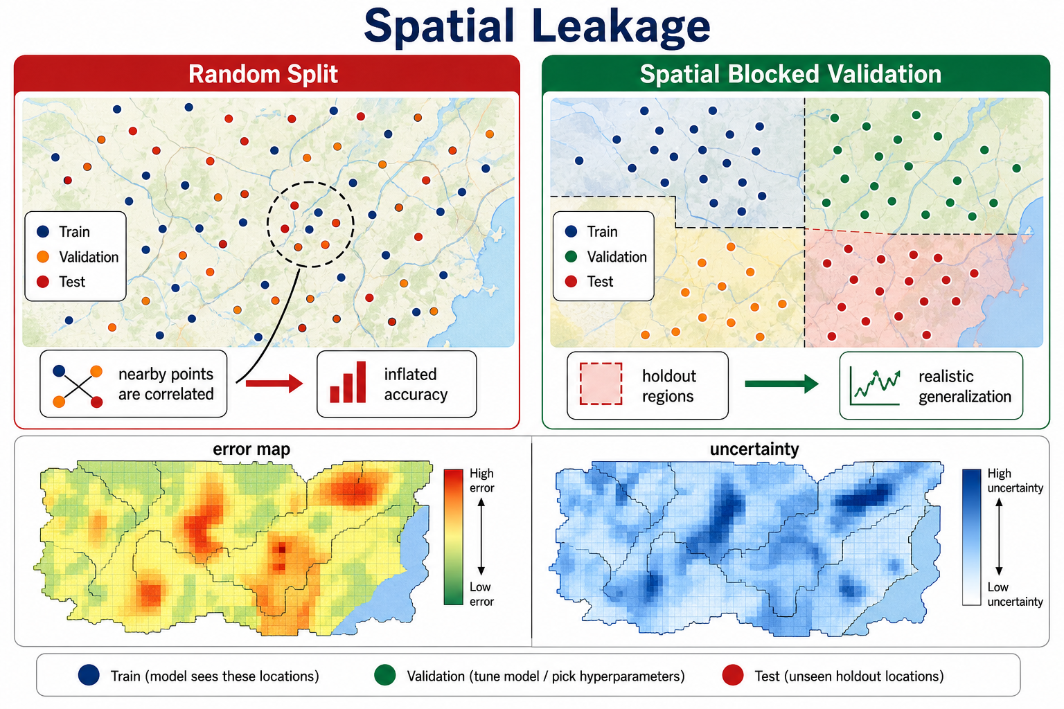
Spatial leakage happens when training and test data are near enough that the model sees almost the same geography in both splits. Random train-test splits can make a model look excellent because nearby points share terrain, roads, climate, sensor artifacts, demographics, or labeling habits. That performance may collapse when the model is moved to a new city, watershed, crop region, country, season, or sensor.

Better evaluation strategies include:

• Spatial blocked validation: hold out entire geographic regions.
• Temporal validation: train on past data and test on future periods.
• Group validation: split by watershed, county, farm, sensor path/row, disaster event, or jurisdiction.
• Leave-one-region-out testing: repeatedly hold out one region to measure transferability.
• Error maps: map where the model fails, not only the global accuracy score.
• Calibration checks: test whether predicted probabilities match observed outcomes.
• Ablation tests: remove location proxies or sensitive features to see what the model relies on.

Research and Standards Foundations

GeoAI should be evaluated with spatial structure in mind. Spatial autocorrelation means random train-test splits can overstate model performance because nearby training and test observations are not independent. Spatial, temporal, blocked, or grouped cross-validation is often more honest when the system will be used in new places or future time periods.

GeoRAG should be treated as both a retrieval system and a geospatial reasoning system. Text similarity alone is not enough. Retrieval should combine semantic relevance with spatial filters, temporal filters, authoritative source ranking, CRS-aware geometry operations, and citations. The answer should expose what was retrieved and what spatial assumptions were applied.

Modern GeoAI research is moving quickly, but the stable engineering lesson is simple: models should be evaluated against the way they will be used. A model meant for national deployment needs geographic holdouts. A model meant for future imagery needs temporal holdouts. A model meant to assist permitting needs authoritative source ranking, jurisdiction boundaries, citations, and human review. A model that produces maps needs map-based residual analysis.

Math

Important math includes spatial autocorrelation, variograms, embeddings, convolution, graph neural networks, attention, vector similarity, hybrid spatial-vector search, ranking, uncertainty estimation, and evaluation metrics. Spatial train-test splits should respect geography, time, and domain shift.

Key computation patterns:

embedding vector:
v = [v1, v2, ..., vd]

cosine similarity:
cosine_similarity(a, b) = dot(a, b) / (||a|| * ||b||)

hybrid GeoRAG scoring:
score(document) =
  alpha * semantic_similarity(query_embedding, document_embedding)
  + beta * text_score(query, document)
  + gamma * spatial_relevance(query_geometry, document_geometry)
  + delta * temporal_relevance(query_time, document_time)
  + epsilon * source_authority(document.source)

spatial candidate filter:
candidate if
  ST_Intersects(document.geometry, query_area)
  and document.time overlaps query_time_window

transformer attention:
Attention(Q, K, V) = softmax((Q * K^T) / sqrt(d_k)) * V

blocked spatial validation:
train_blocks, test_blocks = split_by_region(all_blocks)
model.fit(samples within train_blocks)
evaluate(samples within test_blocks)

Linear algebra is foundational here: embeddings are vectors, similarity is computed over vector space, attention uses matrix multiplication, and GeoRAG adds spatial and temporal filters around semantic retrieval. The geospatial part is not decorative; it changes which documents are eligible to be retrieved.

Spatial feature engineering often combines:

• raw coordinates or safer spatial encodings;
• H3/S2/grid cell features;
• distances to roads, water, schools, hazards, services, or infrastructure;
• neighborhood aggregates within buffers or travel-time areas;
• raster samples from elevation, imagery, weather, land cover, or climate surfaces;
• graph features such as centrality, upstream/downstream relation, or shortest path;
• time features such as season, recurrence interval, lagged values, or event windows.

See also: Math and Algorithms Reference

Tools of the Trade

• ML: scikit-learn, PyTorch, TensorFlow, XGBoost.
• Geospatial ML: TorchGeo, Raster Vision, DeepForest, eo-learn, geemap.
• Retrieval: vector databases, PostGIS, hybrid search, Elasticsearch/OpenSearch.
• Earth observation models: Prithvi, SatMAE, Clay, Segment Anything adaptations, remote sensing foundation models.
• Evaluation: spatial cross-validation, holdout regions, error maps, calibration plots.
• Data and labeling: STAC, COG, GeoParquet, GeoPackage, Label Studio, CVAT, Roboflow, geospatial annotation workflows.
• Serving and monitoring: FastAPI, BentoML, MLflow, model registries, feature stores, dashboards, drift monitors, human review queues.

Examples of Real-World Solutions

• A model detects building footprints from imagery.
• A wildfire risk model combines fuels, weather, terrain, and historical ignitions.
• A graph model predicts road segment congestion.
• A GeoRAG assistant answers questions about a site using maps, permits, hazard layers, and local ordinances.
• A flood model segments water from Sentinel-1 SAR after hurricanes and flags roads likely to be impassable.
• A utility model predicts vegetation encroachment risk by combining LiDAR, imagery, asset location, weather, and maintenance history.
• A city planning model identifies heat-vulnerable blocks using land surface temperature, tree canopy, age, income, building density, and cooling-center access.
• A conservation model detects deforestation and road expansion from time-series satellite imagery.
• A telecom model predicts service gaps from terrain, tower locations, building footprints, demand, and drive-test measurements.
• A GeoRAG assistant for emergency management retrieves shelter locations, flood depths, evacuation zones, road closures, weather alerts, and local procedures.
• A crop-monitoring model uses multispectral imagery, weather, soil, and field boundaries to estimate stress while showing uncertainty by field.
• A transportation model predicts crash risk for road segments using network features, traffic volume, lighting, weather, speed, and prior incidents.

Example GeoAI Design Notes

Building footprint extraction: Use high-resolution imagery and labeled polygons. Train a segmentation model, validate by city or region, post-process masks into polygons, remove slivers, compare against parcel and address data, and send uncertain cases to human review.

Wildfire risk modeling: Combine fuels, slope, aspect, weather, drought indices, historical ignitions, distance to roads, and settlement patterns. Use temporal validation so the model is tested on later fire seasons, and map false negatives because missed high-risk areas are operationally important.

Wildfire GeoAI Mapping Workflow

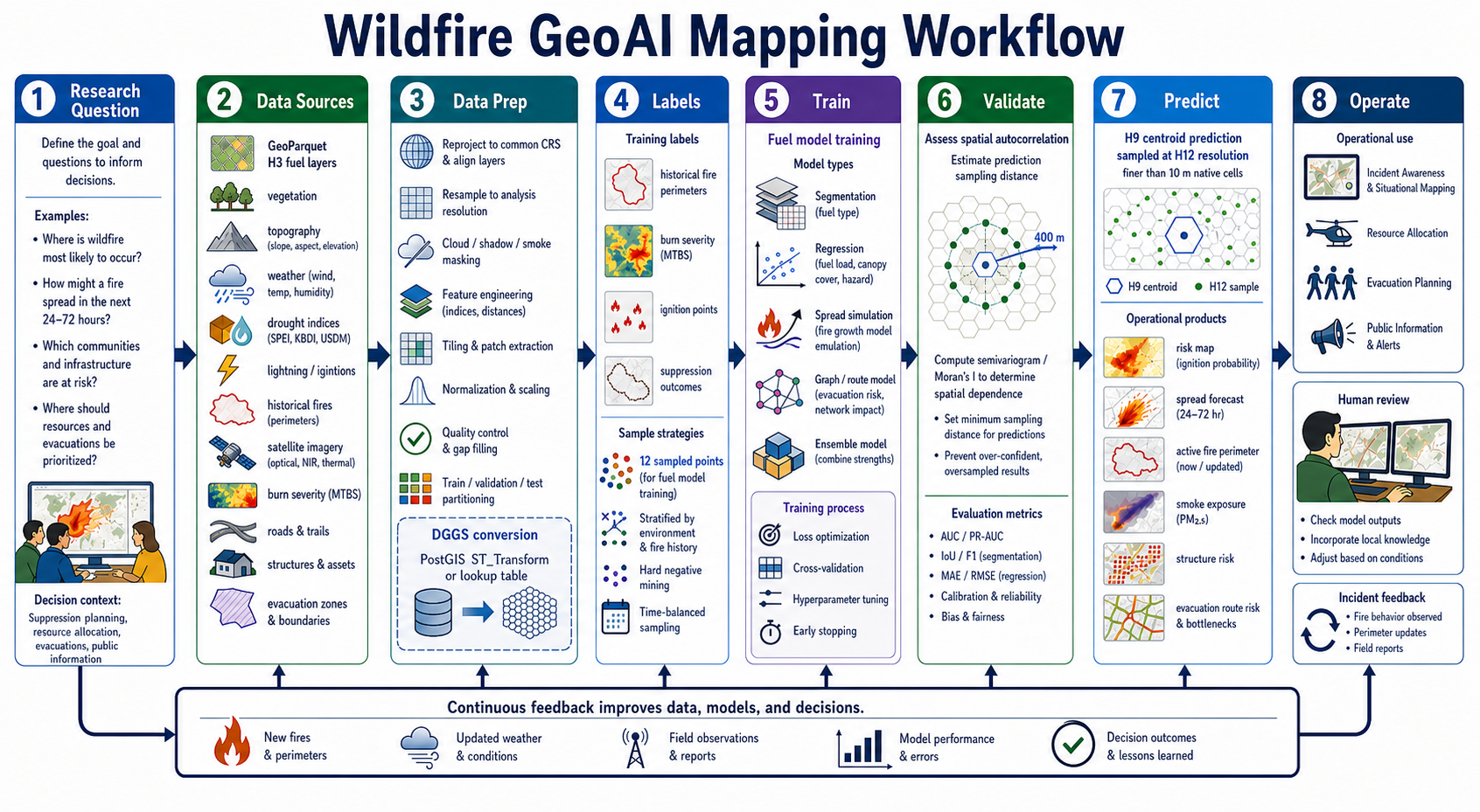
Wildfire mapping is a good GeoAI example because it is both scientific and operational. A useful workflow begins with the decision being supported, not the model architecture. A long-term risk model, a 24-hour spread forecast, an active fire perimeter map, a smoke exposure product, and a structure-risk map all require different data, labels, time windows, and validation.

Common wildfire GeoAI inputs include:

• Fuels and vegetation: LANDFIRE fuel models, vegetation type, canopy cover, canopy height, canopy bulk density, and recent vegetation change.
• Topography: elevation, slope, aspect, terrain position, barriers, drainages, and wind exposure.
• Weather and climate: wind, temperature, humidity, precipitation, drought indices, fuel moisture, lightning, and forecast grids.
• Historical fire records: perimeters, ignition points, suppression history, burn severity, recurrence, seasonality, and fire cause when available.
• Remote sensing: optical, NIR, SWIR, thermal, SAR, active fire detections, smoke, cloud masks, and pre/post-fire imagery.
• Exposure layers: roads, structures, utilities, communities, evacuation zones, shelters, critical facilities, and wildland-urban interface.

Data preparation is usually the largest part of the job. Layers must be reprojected to a common CRS, resampled to an analysis resolution, aligned to a grid, clipped to a study area, time-stamped, quality-masked, and checked for nodata. Time matters: weather at ignition time, fuels before fire, burn severity after fire, and suppression actions during fire should not be mixed casually. A model that accidentally uses post-fire data to predict pre-fire risk is leaking the answer.

Training labels depend on the question:

• Ignition probability: ignition points or historical start locations, often paired with background/non-ignition samples.
• Burn probability or fire occurrence: historical perimeters or simulated fire occurrence grids.
• Spread forecasting: perimeter growth between time steps, active fire detections, weather, fuels, and topography.
• Burn severity: MTBS or field-calibrated severity labels, often using NBR/dNBR-derived products.
• Structure risk: structures inside or near historical perimeters, ember exposure, defensible space, fuels, slope, roads, and response constraints.
• Evacuation risk: road network capacity, fire spread direction, closure likelihood, population, shelters, and travel-time models.

Model choices should match the output. Segmentation models can map burn scars, smoke plumes, or active perimeters from imagery. Regression or classification models can estimate ignition probability, structure risk, or burn probability. Spatiotemporal models can forecast spread under changing weather. Graph models can score evacuation route vulnerability. Ensembles can combine physics-inspired fire behavior models, statistical models, machine learning, and expert rules.

Validation should be spatial, temporal, and event-aware. Hold out entire fires, fire seasons, or regions rather than randomly splitting pixels inside the same fire perimeter. Map false negatives, false positives, calibration, and uncertainty. In wildfire operations, an apparently small false-negative area may matter if it contains a community, evacuation route, powerline, or critical watershed.

Prediction products should be treated as decision-support layers, not automatic decisions. Useful products include risk maps, spread forecasts, active perimeter updates, smoke exposure estimates, structure-risk surfaces, evacuation route risk, uncertainty maps, and error maps. Human review is not a courtesy step; it is part of the system. Incident command observations, field reports, updated perimeters, weather changes, suppression activity, and post-event outcomes should feed back into data quality, labels, model monitoring, and future training.

Crop Insurance GeoAI Workflow

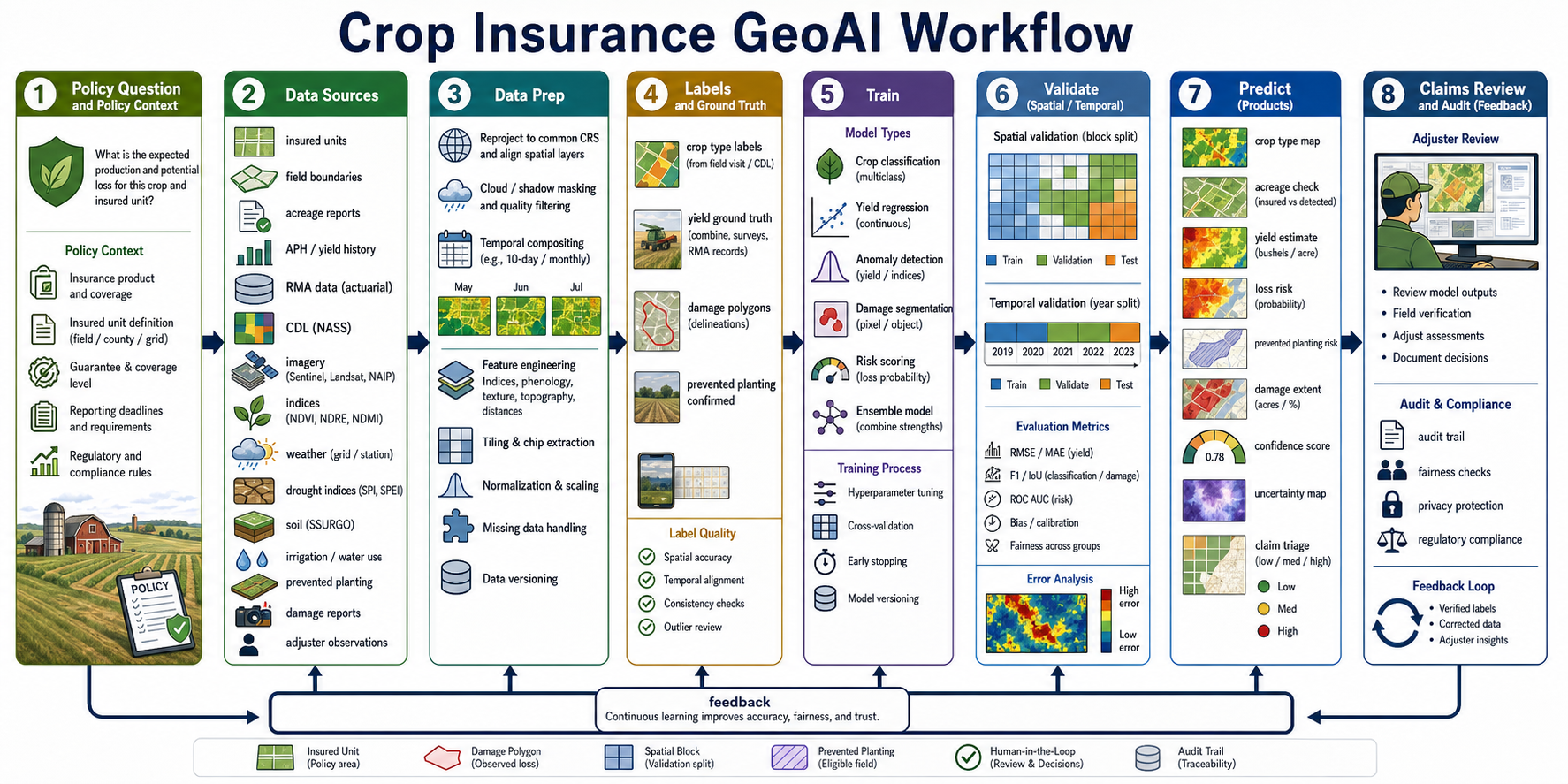
Agricultural crop insurance is another strong GeoAI example because the workflow must connect science, policy, field evidence, actuarial data, remote sensing, and human review. The model is not just predicting crop condition; it is supporting a regulated business process where acreage, crop type, yield, cause of loss, timing, coverage rules, and documentation all matter.

A good crop insurance GeoAI workflow begins with the policy question:

• Is the reported crop type consistent with observed imagery and historical patterns?
• Does the insured acreage match field boundaries, acreage reports, and detectable planted area?
• Is yield loss plausible given weather, drought, crop condition, soil, irrigation, and nearby fields?
• Does imagery support a reported damage event, prevented planting claim, or production shortfall?
• Which claims need adjuster review first because model evidence, uncertainty, or potential loss is high?

Common inputs include:

• Policy and insurance context: insured units, coverage level, crop year, crop type, practice, guarantee, reporting deadlines, and applicable rules.
• Producer and field data: field boundaries, acreage reports, APH/yield history, planting dates, harvest dates, irrigation practice, and prior claims where available.
• USDA and public data: RMA actuarial data, RMA Summary of Business data, NASS Cropland Data Layer, NASS crop progress/condition, SSURGO soils, weather stations, gridded weather, drought indices, and disaster declarations.
• Remote sensing: Sentinel-2, Landsat, MODIS/VIIRS, NAIP, SAR where useful, NDVI, NDRE, NDMI, crop phenology curves, cloud masks, and time-series composites.
• Ground truth: combine records, adjuster observations, field photos, damage polygons, yield monitor or survey data, prevented planting confirmations, and expert review.

Data preparation is where trust is built. Field boundaries must be aligned with imagery, administrative units, and insured-unit definitions. Imagery needs cloud/shadow masking, temporal compositing, crop-calendar alignment, and consistent resolution. Weather and drought variables must be joined to the correct field, county, or grid cell and time window. Yield labels should be checked for outliers, missing values, changed management practices, irrigation differences, and policy-driven reporting effects.

Training targets depend on the product:

• Crop classification: crop type or practice class from imagery, CDL history, phenology, and reported acreage.
• Acreage verification: planted-area detection, boundary consistency, and mismatch scoring.
• Yield estimation: continuous yield or yield anomaly relative to APH, local weather, soil, and phenology.
• Loss risk: probability of yield loss, indemnity risk, drought loss, hail/wind damage, flood damage, or quality loss.
• Damage mapping: affected acres, damage severity, and event timing from imagery and adjuster evidence.
• Prevented planting risk: fields likely affected by excessive moisture, flooding, timing constraints, soil, and local planting progress.
• Claim triage: prioritize claims for review using expected loss, uncertainty, evidence conflict, and compliance rules.

Validation should respect geography, time, crop type, and policy. A model trained on one crop region, irrigation system, crop year, or reporting pattern may not transfer to another. Spatial splits by county or region, temporal splits by crop year, and grouped splits by producer or insured unit help avoid leakage. Evaluation should include RMSE/MAE for yield, F1/IoU for crop or damage maps, calibration for risk scores, and fairness checks across farm size, region, crop type, irrigation status, and data availability.

Prediction products should be decision-support evidence, not automatic claim decisions. Useful outputs include crop type maps, acreage mismatch flags, yield estimates, anomaly maps, loss-risk surfaces, damage extent, prevented planting risk, confidence scores, uncertainty maps, and claim triage queues. Human adjuster review, field verification, documentation, privacy protection, regulatory compliance, and audit trails are part of the model system. Every prediction should preserve data lineage, model version, input dates, CRS, uncertainty, and review outcome.

Conservation and Natural Resource Planning GeoAI Workflow

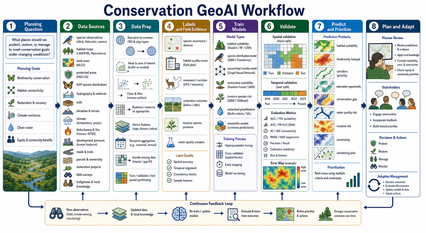
Conservation and natural resource planning uses GeoAI to help decide where to protect, restore, monitor, or manage land and water under changing ecological, social, and climate conditions. The work is not only predictive; it is also values-based and policy-aware. A habitat suitability model, corridor map, restoration priority map, watershed risk model, or invasive species alert should support planner review, community input, and adaptive management rather than replace them.

A good conservation GeoAI workflow starts with a planning question:

• Which places are most important for biodiversity, habitat connectivity, clean water, climate resilience, or restoration?
• Where are species, habitats, wetlands, watersheds, or protected areas most vulnerable to disturbance?
• Which restoration projects are likely to improve habitat, water quality, fire resilience, carbon storage, or community benefits?
• Where are conservation gaps between current protected areas and future ecological needs?
• How should limited funding, field crews, or monitoring effort be prioritized?

Common inputs include:

• Species and habitat evidence: species observations, survey records, camera traps, acoustic sensors, telemetry, nest sites, absence/background samples, habitat quality scores, and expert review.
• Land and water context: land cover, vegetation, wetlands, hydrography, watersheds, floodplains, soils, geology, elevation, slope, aspect, riparian buffers, and water quality samples.
• Conservation and ownership layers: protected areas, PAD-US, easements, parcels, ownership, public lands, management units, restoration projects, and stewardship boundaries.
• Pressure and disturbance: roads, trails, development pressure, human footprint, fire history, invasive species, timber harvest, grazing, mining, recreation, drought, and climate projections.
• Community and governance: local knowledge, Indigenous knowledge where shared under appropriate governance, access constraints, equity priorities, policy boundaries, and stakeholder feedback.

Data preparation must preserve ecological meaning. Species observations need spatial accuracy checks, duplicate handling, sampling-bias review, and temporal filtering. Habitat and land-cover layers must be aligned by CRS, resolution, classification scheme, season, and date. Absence data is especially difficult: no observation is not always evidence that a species is absent. Planning layers also have legal and social meaning, so ownership, protected status, and access restrictions must be current and cited.

Training labels depend on the planning product:

• Habitat suitability: species presence/background, field plots, habitat quality scores, vegetation, climate, terrain, and disturbance features.
• Species distribution models: occurrence data, pseudo-absence/background sampling, climate variables, land cover, topography, and sampling effort.
• Connectivity and corridors: movement tracks, resistance surfaces, roads, barriers, protected patches, streams, ridgelines, and graph/circuit metrics.
• Restoration suitability: past restoration outcomes, degraded areas, soils, hydrology, ownership, cost, feasibility, and climate resilience.
• Invasive species risk: occurrence reports, propagule pressure, roads/trails, disturbance, climate, waterways, and survey effort.
• Watershed prioritization: water quality samples, land cover, erosion risk, slope, riparian condition, impervious surface, agriculture, and upstream/downstream relationships.
• Conservation gap analysis: protected areas, species ranges, habitat quality, climate refugia, management status, and representation targets.

Model choices should match the ecological process and planning use. Tree-based models and generalized additive models are common for tabular habitat suitability. CNNs and transformers can map land cover, wetlands, canopy, or disturbances from imagery. Graph neural networks, least-cost paths, circuit theory, and resistance models can support connectivity. Multi-criteria decision analysis and optimization can combine predictions with cost, ownership, feasibility, equity, and policy constraints.

Validation should be spatial, temporal, taxonomic, and sampling-aware. Hold out regions, watersheds, ecoregions, survey years, or monitoring projects. Test whether models generalize to unsampled areas and future conditions. Report AUC or PR-AUC carefully, but also map residuals, omission errors, commission errors, calibration, uncertainty, and bias from uneven sampling. In conservation, a false negative can mean overlooking a critical habitat patch; a false positive can redirect limited restoration resources away from better sites.

Prediction products should be planning evidence. Useful outputs include habitat suitability maps, species distribution maps, biodiversity hotspot maps, corridor priorities, restoration opportunity maps, conservation gap maps, watershed risk layers, invasive species risk surfaces, uncertainty maps, and monitoring plans. Planner review should incorporate field feasibility, stewardship capacity, community priorities, equity, cost, legal constraints, and local ecological knowledge. After implementation, monitoring outcomes should feed back into labels, model updates, and adaptive management.

Utility Resource Mapping GeoAI Workflow

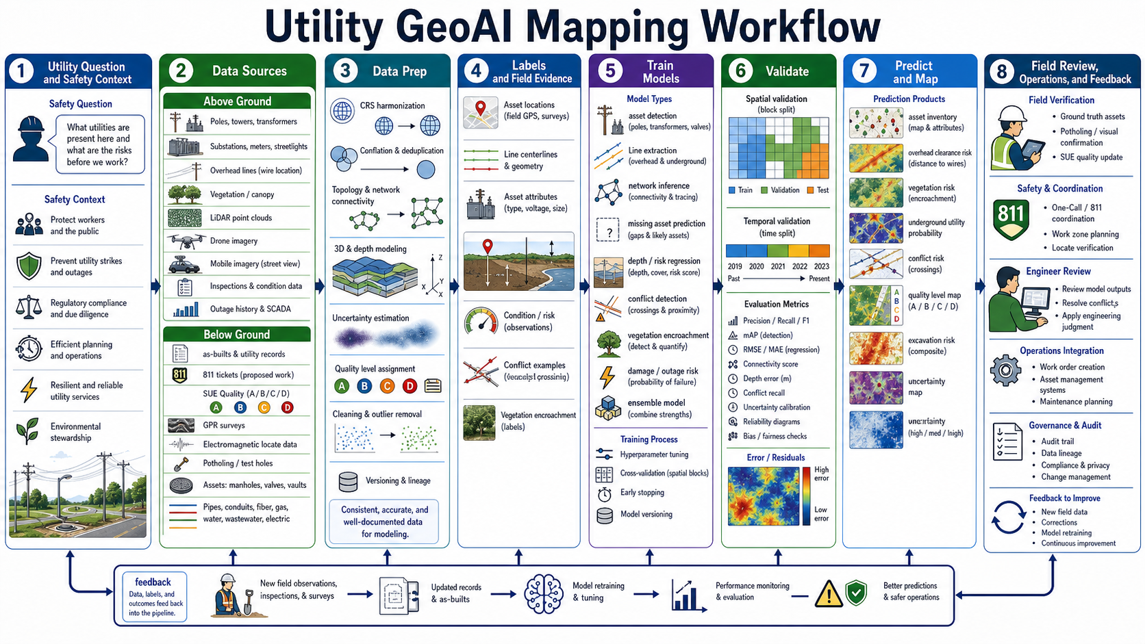
Utility resource mapping uses GeoAI to improve asset inventories, work planning, risk assessment, and field verification for above-ground and below-ground infrastructure. The stakes are high: utility maps support worker safety, public safety, excavation planning, outage response, vegetation management, engineering design, regulatory compliance, and environmental stewardship. A prediction should never be treated as permission to dig or work near energized assets; it is evidence that must be reviewed with field verification, engineering judgment, and utility-owner procedures.

A good utility GeoAI workflow starts with the safety and operations question:

• Which assets are present, missing, duplicated, outdated, or incorrectly located?
• Where are overhead clearance, vegetation encroachment, pole condition, or outage risks increasing?
• Where might underground utilities conflict with proposed excavation, design, or construction work?
• Which records need field verification because confidence is low or consequences are high?
• How should work orders, inspections, locate requests, and maintenance crews be prioritized?

Above-ground utility inputs often include:

• Electric and telecom assets: poles, towers, transformers, substations, cabinets, meters, streetlights, antennas, and overhead conductors.
• Imagery and 3D capture: aerial imagery, drone imagery, mobile imagery, LiDAR point clouds, oblique imagery, thermal imagery, and inspection photos.
• Operational records: asset management systems, outage history, SCADA or telemetry, maintenance logs, inspection condition scores, vegetation work history, and work orders.
• Context layers: parcels, roads, rights-of-way, land cover, canopy, terrain, access constraints, weather exposure, and customer/service areas.

Below-ground utility inputs often include:

• Records and engineering data: as-builts, CAD drawings, GIS utility records, asset registries, design plans, service tickets, and construction records.
• Locate and SUE evidence: 811/one-call tickets, electromagnetic locate data, ground penetrating radar, test holes/potholing, exposed utility observations, survey measurements, and Subsurface Utility Engineering quality levels.
• Network assets: water pipes, wastewater lines, stormwater, gas, electric, telecom, fiber, conduits, valves, manholes, vaults, meters, hydrants, laterals, and abandoned assets.
• 3D and depth context: cover depth, vertical datum, surface elevation, pipe diameter, material, installation date, confidence, and uncertainty.

Data preparation is the hard part. Utility records are often old, duplicated, incomplete, or stored in mixed CAD, GIS, PDF, spreadsheet, and work-management systems. Data prep must reconcile CRS, units, vertical reference, asset IDs, topology, connectivity, snapping tolerance, version history, ownership, and quality level. Below-ground mapping must preserve uncertainty explicitly: an approximate line from a legacy drawing is not the same as a surveyed test hole.

Training labels depend on the mapping product:

• Asset detection: labeled poles, transformers, valves, manholes, meters, cabinets, or streetlights from imagery, LiDAR, and surveys.
• Line extraction: overhead conductor paths, buried utility alignments, pipe centerlines, trench scars, or probable corridors.
• Network inference: missing connections, disconnected segments, laterals, service lines, and topology errors.
• Depth and cover estimation: depth regression from SUE evidence, as-builts, terrain, installation patterns, and field measurements.
• Conflict detection: crossings, proximity to proposed work, clearance violations, unknown-quality utilities, and high-consequence conflicts.
• Vegetation and condition risk: encroachment near overhead lines, leaning poles, damaged equipment, access constraints, and outage probability.
• Excavation and damage risk: combined risk from utility uncertainty, locate quality, project scope, soil, traffic, asset criticality, and historical damage.

Model choices should reflect both asset type and evidence quality. Object detection and segmentation models can extract visible assets from imagery or LiDAR. Graph models can infer connectivity and trace networks. Regression models can estimate depth, cover, clearance, or risk. Anomaly detection can find missing assets, improbable geometry, mismatched attributes, or unexpected service areas. Ensembles can combine records, field evidence, imagery, and engineering rules.

Validation should be field-aware and consequence-aware. Spatial blocked validation helps avoid overfitting to a single city, utility owner, neighborhood design pattern, or imagery campaign. Below-ground models should be evaluated separately by SUE quality level, asset type, depth range, material, and locate method. Useful metrics include precision/recall/F1 for detection, mAP for object detection, topology/connectivity scores, RMSE/MAE for depth or clearance, conflict recall, calibration, and error maps. High-consequence false negatives deserve special review.

Prediction products should make uncertainty and evidence visible. Useful outputs include asset inventory updates, missing-asset candidates, overhead clearance risk, vegetation encroachment risk, probable underground utility corridors, quality-level maps, conflict risk, excavation risk, outage risk, uncertainty maps, and work-order priority queues. Field verification, SUE updates, engineer review, 811 coordination, audit trails, and feedback from completed work should continuously improve the data and models.

Medical Indoor GIS and Emergency Routing GeoAI Workflow

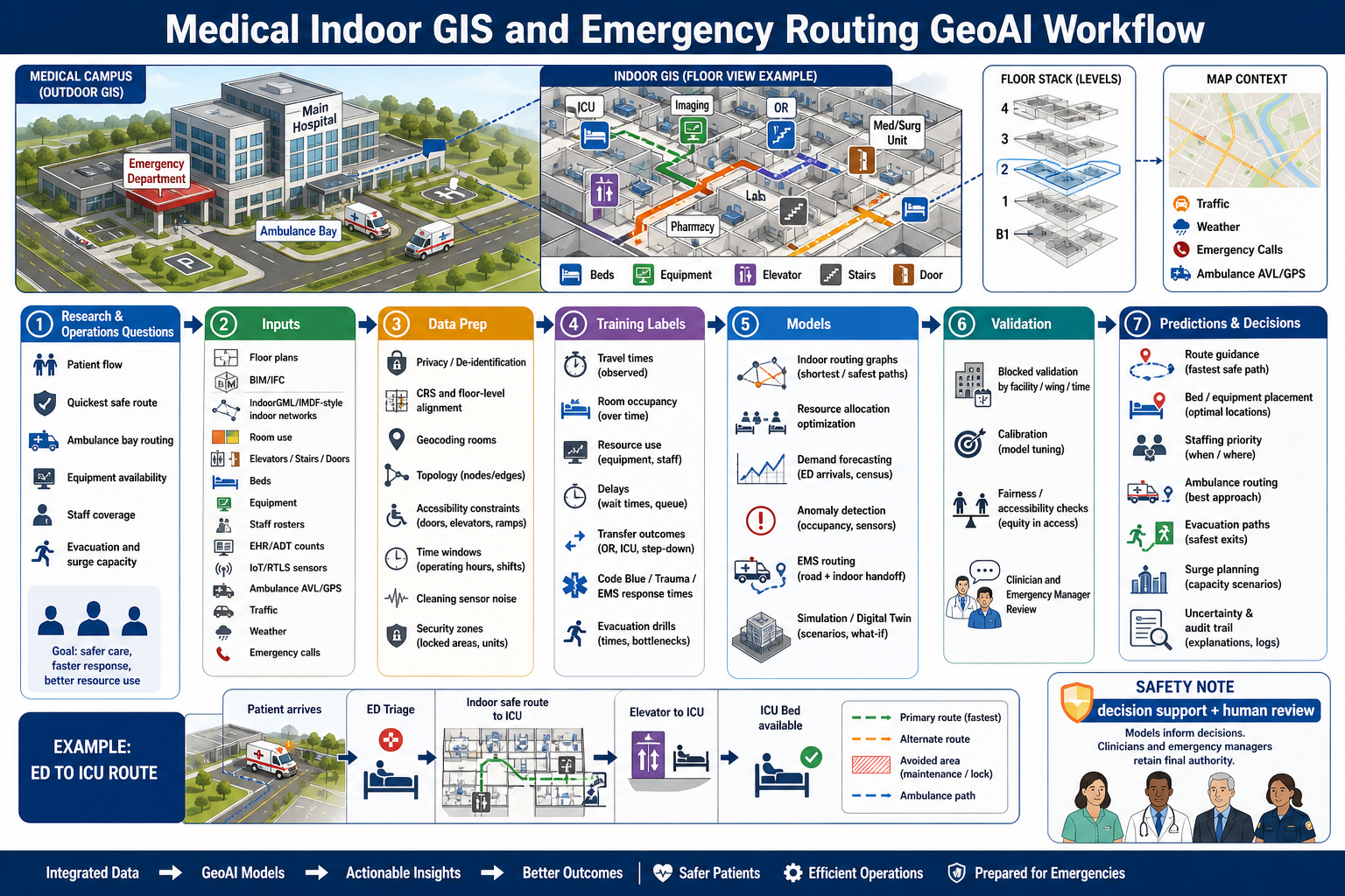
Medical geography is not only about disease maps and public health regions. Inside hospitals, clinics, laboratories, long-term care facilities, and emergency operations centers, location affects patient safety, staff workload, resource access, evacuation, ambulance routing, and response time. Indoor GIS and GeoAI can help connect building maps, real-time operations, transportation networks, and emergency management into a decision-support system.

A good medical GeoAI workflow starts with the operational and ethical question:

• How can patients, staff, visitors, and emergency responders move through a facility safely and quickly?
• Which route is fastest, accessible, clinically appropriate, and allowed under current security or infection-control constraints?
• Where should beds, wheelchairs, ventilators, monitors, medication carts, blood products, or mobile imaging units be staged?
• Which departments are likely to experience crowding, transfer delay, or resource shortage?
• How should ambulances route to the correct entrance, bay, floor, or specialty unit during normal operations, mass casualty events, or facility disruptions?
• How can evacuation and shelter-in-place plans account for patients who need oxygen, dialysis, neonatal care, isolation, bariatric transport, or multiple staff escorts?

Common inputs include:

• Indoor GIS and building data: floor plans, BIM/IFC models, room numbers, departments, doors, elevators, stairs, ramps, corridors, restricted areas, clean/dirty paths, fire compartments, exits, and IndoorGML-style navigation networks.
• Clinical and operational data: bed status, patient census, admission/discharge/transfer events, staffing, equipment location, supply inventory, procedure schedules, lab and imaging queues, environmental services status, and surge plans.
• Positioning and sensor data: RTLS tags, Wi-Fi/Bluetooth positioning, badge systems, equipment telemetry, elevator status, occupancy sensors, nurse call systems, and security access logs.
• Outdoor and emergency context: ambulance AVL/GPS, street networks, traffic, weather, emergency calls, road closures, helipad access, mutual-aid facilities, shelters, and regional hospital capacity.
• Policy and safety constraints: HIPAA/privacy rules, access control, infection control, accessibility requirements, hazardous materials, visitor restrictions, incident command rules, and cybersecurity controls.

Data preparation must handle privacy and topology at the same time. Patient and staff data should be minimized, de-identified where possible, access-controlled, logged, and governed by clinical policy. Spatial data needs floor-level alignment, room geocoding, indoor network topology, vertical routing between floors, elevator constraints, accessible paths, one-way or restricted corridors, security zones, and time-dependent closures. Sensor streams need timestamp alignment, noise filtering, missing-data handling, and clear separation between observed movement and inferred movement.

Training labels depend on the decision being supported:

• Indoor routing: observed travel times, transfer paths, door/elevator waits, blocked corridors, accessibility constraints, and staff escort requirements.
• Resource allocation: equipment use, bed turnover, supply demand, staffing levels, queue times, department census, and surge-event history.
• Emergency response: code blue response times, trauma team activation, ambulance-to-bed intervals, evacuation drill performance, shelter-in-place actions, and incident command logs.
• Patient flow: arrival volumes, triage acuity, admission probability, discharge timing, transfer delays, and bottlenecks between departments.
• Facility risk: outage history, utility dependencies, isolation rooms, negative-pressure rooms, oxygen zones, generators, and critical equipment dependencies.

Model choices should match clinical risk. Routing can use indoor graph algorithms, time-dependent shortest paths, accessibility-aware path finding, and simulation. Resource allocation can use optimization, queueing models, forecasting, reinforcement learning under strict guardrails, or digital twins. Emergency services routing can combine outdoor network routing with indoor handoff routing from ambulance bay to unit. Anomaly detection can flag unusual crowding, equipment loss, elevator failures, or response delays.

Validation should include clinicians, emergency managers, facilities staff, accessibility experts, security teams, and privacy officers. Hold out facilities, floors, wings, shifts, seasons, drills, or events rather than relying only on random samples. Useful metrics include route travel-time error, accessibility compliance, resource forecast calibration, queue-time error, response-time recall for high-acuity cases, evacuation bottleneck detection, and fairness checks for patients with mobility, language, disability, or isolation needs.

Prediction products should be operational evidence, not automatic clinical orders. Useful outputs include indoor route guidance, accessible evacuation paths, ambulance routing, equipment staging maps, bed and staffing priority queues, surge capacity scenarios, transfer bottleneck maps, isolation-routing plans, uncertainty maps, and audit trails. Human review is essential because the model may not know that an elevator is reserved, a corridor is contaminated, a patient needs special equipment, or an emergency manager has changed the incident plan.

Genetic Lineage Mapping of Domesticated Species GeoAI Workflow

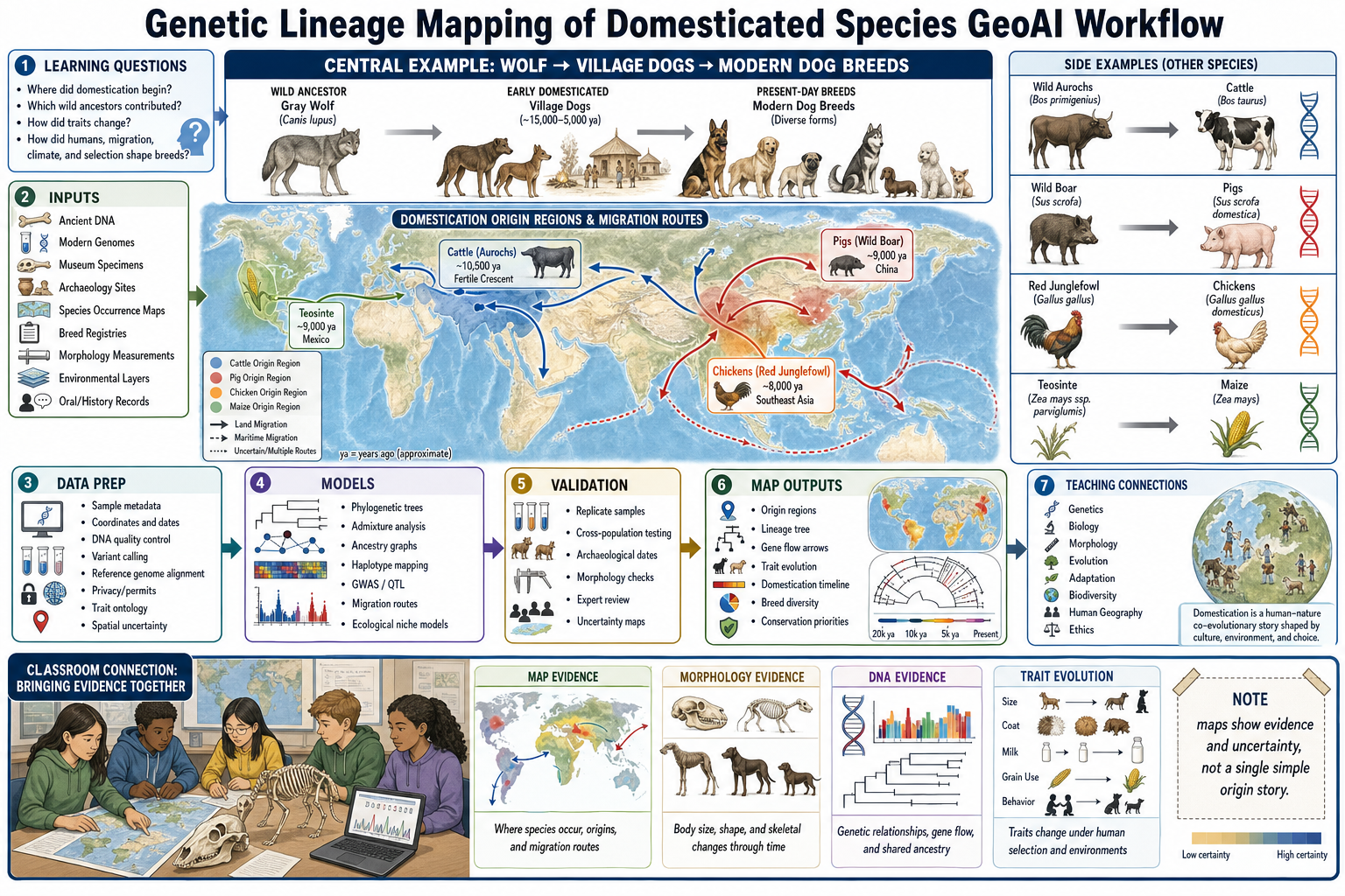
Genetic lineage mapping connects geography, DNA, archaeology, morphology, ecology, and human history. Instead of mapping only where a species lives today, the workflow asks how wild ancestors, ancient populations, human movement, selection, and environments produced present-day domesticated species and breeds. This is a powerful teaching example because students can see that biology is spatial: genes move, traits change, species adapt, and people shape landscapes and lineages.

A good domestication mapping workflow starts with learning and research questions:

• Where did domestication likely begin, and was there one origin or several?
• Which wild ancestor populations contributed to present-day domesticated breeds or varieties?
• How did migration, trade, climate, ecology, and human selection change the lineage through time?
• Which traits changed most visibly in morphology, behavior, productivity, disease resistance, or adaptation?
• How can mapped evidence teach genetics, biology, morphology, evolution, biodiversity, conservation, and ethics?

Common inputs include:

• Genetic evidence: ancient DNA, modern genomes, mitochondrial DNA, Y-chromosome markers, SNPs, haplotypes, structural variants, reference genomes, and breed or variety panels.
• Specimen and field evidence: museum specimens, archaeological remains, radiocarbon dates, zooarchaeology, herbarium records, species occurrence points, field surveys, and wild-relative populations.
• Morphology and traits: body size, skull shape, horn shape, coat color, ear form, seed size, grain shattering, milk production, behavior, fertility, disease resistance, and environmental tolerance.
• Spatial and historical context: archaeological site maps, migration routes, trade networks, climate reconstructions, land cover, elevation, ecological niche layers, settlement patterns, and historical records.
• Teaching materials: simplified maps, lineage trees, trait timelines, classroom datasets, photographs, skeletal diagrams, ethical discussion prompts, and uncertainty legends.

Data preparation must preserve both biological and geographic meaning. Samples need metadata for species, breed, specimen ID, collection method, age, date, location, uncertainty, permissions, and cultural or Indigenous data governance. DNA workflows require quality control, contamination checks, reference-genome alignment, variant calling, missing-data handling, and reproducible pipelines. Morphology needs consistent measurements and trait definitions. Spatial layers need CRS alignment, temporal context, and uncertainty because ancient sample locations and inferred origins are rarely exact points.

Training labels and targets depend on the lesson or research product:

• Ancestry and lineage: wild ancestor groups, domestic populations, breed groups, admixture components, and ancient-to-modern relationships.
• Origin and spread: probable domestication regions, migration routes, time slices, archaeological phases, and gene-flow corridors.
• Trait evolution: genotype-trait associations, morphology changes, selection signatures, breed-defining traits, and adaptation to climate or management.
• Wild-relative comparison: overlap between modern breeds and wild ancestor ranges, remaining wild diversity, introgression, and conservation priorities.
• Classroom explanation: simplified evidence layers that let students compare map evidence, DNA evidence, morphology evidence, and historical evidence.

Model choices can include phylogenetic trees, haplotype networks, admixture models, ancestry graphs, GWAS/QTL mapping, ecological niche models, spatial clustering, and temporal visualizations. GeoAI can help by integrating genetic embeddings, trait measurements, mapped environments, and archaeological context. For teaching, the goal is not to hide complexity; it is to make complexity visible enough that learners can reason from evidence.

Validation should avoid oversimplified origin stories. Ancient DNA, modern genomes, morphology, archaeology, and geography should be checked against one another. Hold out populations, regions, time periods, or breeds when testing prediction models. Report uncertainty for ancestry proportions, origin regions, migration arrows, trait associations, and sample bias. A map should show that domestication can involve multiple origins, extinct ancestor lineages, later admixture, backcrossing with wild relatives, and human movement.

Prediction and teaching products include origin-region maps, genetic lineage trees, gene-flow arrows, domestication timelines, breed diversity maps, morphology comparison panels, trait-evolution maps, wild-relative conservation maps, and classroom activities. Students can compare wolves and modern dog breeds, wild boar and pigs, aurochs and cattle, red junglefowl and chickens, teosinte and maize, or other local examples. The core lesson is that present-day breeds are living maps of inheritance, environment, selection, migration, and human culture.

Business and Medical Facility Site Selection GeoAI Workflow

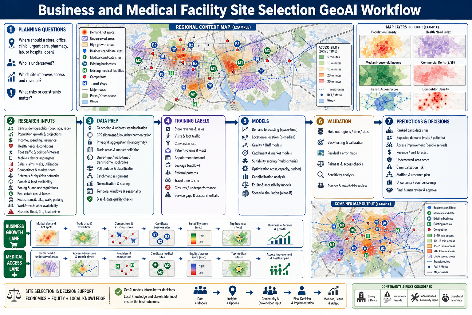
Site selection is one of the classic places where GIS, business analytics, public health, transportation, real estate, and GeoAI meet. The same mapping logic can help a company decide where to open a store, office, warehouse, pharmacy, urgent care clinic, outpatient lab, or hospital. The best site is rarely just the cheapest parcel or the place with the highest population. It is a location where demand, access, competition, cost, equity, regulations, risk, staffing, and long-term growth fit the mission.

A good site-selection GeoAI workflow starts with the decision question:

• Where should a new business, clinic, urgent care center, pharmacy, laboratory, or hospital be located?
• Which communities are underserved by existing services?
• Which candidate site improves access, revenue, patient volume, or operational resilience?
• How will a new location affect existing stores, clinics, referral networks, and service areas?
• Which real estate, zoning, hazard, transportation, workforce, equity, or community constraints matter?

Common inputs include:

• Market and population data: census demographics, household income, age, population growth, employment, daytime population, consumer spending, insurance coverage, language, disability, vehicle access, and social vulnerability.
• Business and healthcare demand: sales, transactions, loyalty data, appointment demand, patient visits, claims, referrals, leakage, payer mix, wait times, service-line utilization, and unmet need indicators.
• Mobility and access: roads, traffic, transit, walkability, bike access, parking, drive-time areas, walk-time areas, transit-time areas, mobile-device aggregates where legally and ethically usable, and travel-time reliability.
• Competition and complementarity: existing stores, clinics, hospitals, pharmacies, labs, specialists, referral partners, anchor tenants, schools, employers, competitors, and substitutes.
• Site and regulatory context: parcels, zoning, land use, lease or purchase cost, building size, utilities, broadband, workforce availability, environmental constraints, flood/fire/heat risk, permits, and community plans.

Data preparation is where many site-selection models become trustworthy or misleading. Addresses and points of interest must be geocoded, deduplicated, classified, and time-stamped. Candidate parcels need zoning, ownership, access, cost, hazard, and buildability attributes. Demand must be aggregated to privacy-safe geographies, normalized by population or households when appropriate, and aligned to the correct service area. Travel-time surfaces should use realistic networks, not simple circles, especially for emergency care, transit-dependent communities, or rural access.

Training labels depend on the use case:

• Retail or service demand: revenue, visits, conversion rate, repeat customers, market share, basket size, and closure or underperformance history.
• Medical facility demand: patient volume, appointment backlog, travel time, service-line demand, referral leakage, emergency department visits, avoidable utilization, and population health needs.
• Accessibility and equity: underserved-area scores, provider-to-population ratios, travel burden, transit access, social vulnerability, disability access, and language or cultural access.
• Cannibalization and network effects: revenue shift from nearby sites, patient redistribution, referral network changes, and capacity relief at existing facilities.
• Operational feasibility: staffing availability, construction or lease timeline, parking, loading, utilities, broadband, hazard exposure, and local policy constraints.

Model choices should combine market logic and spatial logic. Gravity and Huff-style models estimate probabilistic trade areas by combining attractiveness, travel cost, and competing alternatives. Location-allocation and p-median models help place facilities to minimize travel burden or maximize covered demand under capacity constraints. Forecasting models estimate future visits, sales, or patient volume. Suitability models combine weighted criteria such as access, demand, cost, risk, equity, and regulation. Optimization and scenario simulation can compare candidate portfolios under budget, staffing, and service-area constraints.

Validation should be spatial, temporal, and scenario-aware. Hold out regions, store openings, clinic openings, years, or market areas. Compare predicted revenue, visits, patient volume, travel time, and access improvement against observed outcomes. Map residuals to see where the model overestimates affluent areas, underestimates rural demand, misses transit barriers, or ignores cultural access. Sensitivity analysis is important because small changes in travel-time assumptions, competitor attractiveness, real estate cost, or population growth can change the ranking of candidate sites.

Prediction products should support deliberation. Useful outputs include ranked candidate sites, trade areas, drive-time and transit-time maps, expected revenue or visits, patient-volume forecasts, underserved-area scores, access-improvement maps, cannibalization risk, staffing plans, resource plans, hazard exposure, uncertainty maps, and scenario dashboards. Business leaders, planners, clinicians, community members, real estate teams, and local officials should review the outputs because the final decision blends economics, equity, feasibility, and local knowledge.

Gaussian Splatting GeoAI Mapping Workflow

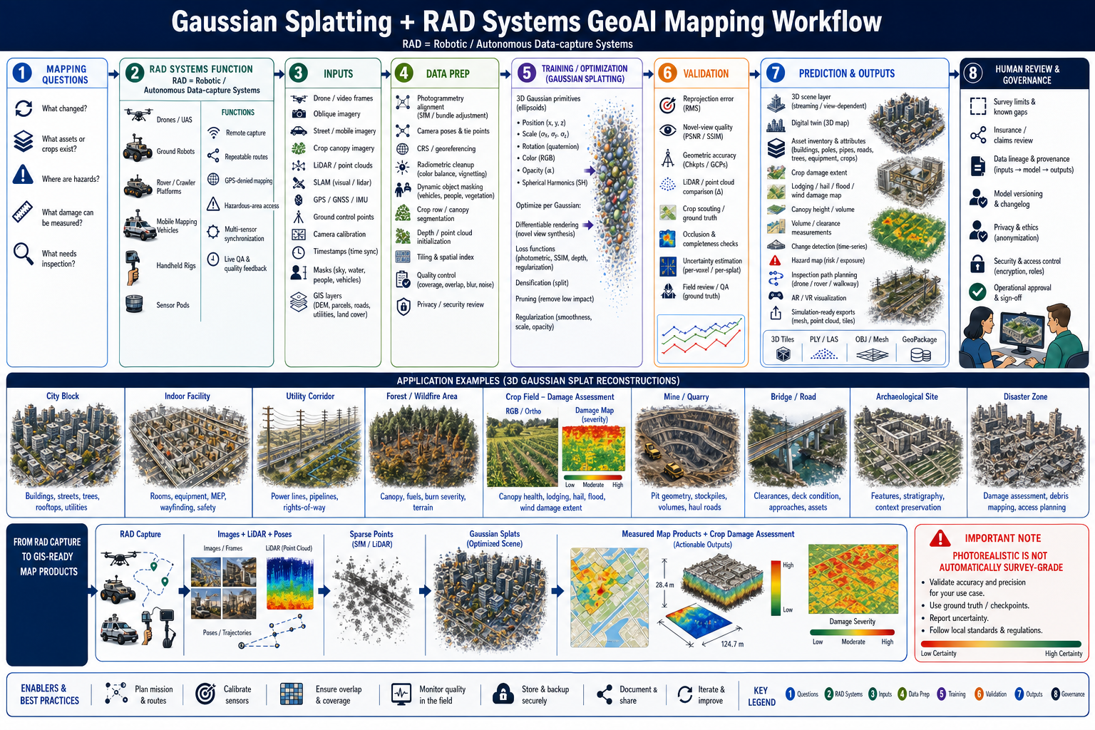
3D Gaussian Splatting is a fast-growing scene reconstruction technique that represents a place as many optimized 3D Gaussian primitives rather than only as a mesh, raster, or point cloud. Each Gaussian can carry position, scale, rotation, opacity, and view-dependent color. For geospatial work, this matters because a photorealistic scene can become an interactive 3D map product for inspection, measurement, simulation, digital twins, and field planning. The caution is just as important: photorealistic is not automatically survey-grade.

In this workflow, RAD systems means Robotic/Autonomous Data-capture systems: drones/UAS, ground robots, rover or crawler platforms, mobile mapping vehicles, handheld rigs, and sensor pods that collect imagery, LiDAR, GNSS/IMU, SLAM, timestamps, and field QA observations. Their function is to make capture repeatable, safer, more complete, and better synchronized than one-off manual image collection. RAD systems are especially useful when the mapping area is hazardous, too large for manual survey, GPS-denied, operationally active, or needs repeated monitoring through time.

A good Gaussian Splatting mapping workflow starts with the mapping question:

• What has changed since the last capture?
• Which assets, structures, vegetation, utilities, roads, rooms, or hazards are visible?
• Which measurements are needed: height, clearance, volume, distance, slope, obstruction, damage, or access?
• Which areas are occluded, uncertain, or need field inspection?
• How should a 3D reconstruction connect back to authoritative GIS layers, survey control, and operational decisions?

Common application areas include:

• Urban and campus digital twins: reconstruct streets, buildings, sidewalks, trees, signs, poles, facades, roofs, courtyards, and public spaces for planning and visualization.
• Indoor and facility mapping: capture rooms, corridors, equipment, MEP systems, labs, warehouses, hospitals, factories, and emergency routes.
• Utility and transportation corridors: inspect power lines, substations, pipelines, bridges, rail, roads, rights-of-way, clearances, vegetation encroachment, and maintenance access.
• Natural resources and hazards: map forests, fuels, burn severity, landslides, flood damage, coastal erosion, mines, quarries, stockpiles, and terrain change.
• Remote crop damage assessment: reconstruct crop canopies and field rows after hail, wind, flood, drought, lodging, pest, disease, or equipment damage to estimate damage extent, canopy height/volume, severity, and inspection priorities.
• Cultural heritage and archaeology: preserve sites, structures, excavation contexts, stratigraphy, artifacts, and visitor interpretation scenes.
• Emergency response and insurance: document debris, damaged buildings, blocked access, post-event conditions, and recovery progress.

RAD systems support those applications in different ways:

• Drones/UAS: capture roofs, bridges, towers, construction sites, disaster zones, forests, crop fields, and inaccessible slopes with planned overlap and repeatable flight paths.
• Ground robots and rovers: enter tunnels, industrial plants, utility corridors, damaged buildings, mines, warehouses, or hazardous areas where human inspection is risky.
• Mobile mapping vehicles: collect street-level imagery, LiDAR, GNSS/IMU, and pavement or asset observations across transportation networks and city blocks.
• Handheld rigs and sensor pods: capture indoor rooms, tight spaces, archaeological contexts, equipment rooms, and places where large platforms cannot operate.
• Autonomous mission software: plans coverage, checks image overlap, synchronizes sensors, flags blur or missing coverage, and stores capture metadata for later audit.

Common inputs include RAD-captured drone video, oblique imagery, street-level or mobile imagery, crop canopy imagery, LiDAR or point clouds, SLAM trajectories, GNSS/IMU observations, ground control points, camera calibration, timestamps, masks, existing DEMs, building footprints, parcels, field boundaries, crop type, planting date, roads, asset layers, and inspection records. Gaussian Splatting does not remove the need for photogrammetry and geodesy; it depends on camera poses, tie points, scale, and spatial reference discipline.

Data preparation usually includes:

• Photogrammetric alignment: structure-from-motion, bundle adjustment, camera pose estimation, tie points, image overlap checks, and calibration review.
• Geospatial control: CRS assignment, ground control points, checkpoints, vertical datum handling, scale constraints, and alignment to GIS layers.
• Image and sensor cleanup: exposure balancing, blur detection, radiometric cleanup, rolling-shutter review, depth initialization, LiDAR fusion, and sensor time synchronization.
• Scene filtering: dynamic object masking for people, vehicles, clouds, water, smoke, reflections, vegetation motion, and construction activity.
• Crop damage prep: align field boundaries, crop rows, canopy masks, pre-event imagery, post-event imagery, scouting notes, weather event timing, and crop growth stage.
• RAD mission QA: check flight logs, robot paths, sensor health, overlap, speed, altitude, safety geofences, battery interruptions, lost tracking, and repeated-pass consistency.
• Production tiling: split large areas into tiles, blocks, levels of detail, streaming packages, and spatial indexes so the scene can load in operational viewers.
• Governance review: privacy, restricted facilities, critical infrastructure, faces, license plates, sensitive assets, and cybersecurity controls.

Training and optimization are different from ordinary supervised classification. A Gaussian scene is optimized so rendered views match the source imagery. The system adjusts the primitives' position, scale, rotation, opacity, and color parameters using differentiable rendering and image losses. Densification adds detail where the reconstruction needs more primitives; pruning removes primitives that add little value or create artifacts. Regularization can encourage smoothness, stable scale, depth consistency, or better geometry.

Validation should be explicit because a visually impressive reconstruction can still be wrong for measurement. Useful checks include reprojection error, held-out view quality, checkpoint accuracy, comparison to LiDAR or survey control, geometric error by asset type, occlusion maps, uncertainty maps, scale drift, temporal consistency, crop scouting or adjuster observations, and field review. If the output will support engineering, public safety, legal evidence, construction, utilities, crop insurance, or emergency response, the workflow needs documented accuracy limits and human approval.

Prediction and output products can include 3D scene layers, digital twin views, asset inventories, volume calculations, clearance measurements, crop damage extent, lodging/hail/flood/wind severity maps, canopy height or canopy volume estimates, change detection, damage maps, hazard maps, inspection paths, AR/VR scenes, training simulations, mesh exports, point cloud exports, and GIS-ready annotations. The best products keep lineage visible: input dates, sensor sources, camera poses, CRS, model version, control points, validation results, uncertainty, and known blind spots.

GeoRAG permitting assistant: Store parcels, zoning, flood zones, overlays, ordinances, permits, and metadata. Retrieve by parcel geometry and jurisdiction first, then semantic relevance. The answer should include citations, map evidence, date of source, and a warning that official staff review is required.

Working Practice Examples

1. Train a simple land-cover classifier and evaluate it with random and spatial splits.
2. Build a hybrid retrieval query that combines text similarity with a bounding-box filter.
3. Create an error map for model predictions.
4. Design a GeoRAG prompt that requires citations to retrieved spatial sources.
5. Label ten image chips for a small segmentation problem and document label uncertainty.
6. Compare random, spatial blocked, and temporal validation scores for the same model.
7. Build a simple place embedding table for neighborhoods or grid cells and search for similar places.
8. Design a human-review workflow for model outputs that affect permitting, safety, or public services.
9. Write a model card for a GeoAI model including CRS, sensors, region, time period, labels, validation split, limitations, and intended use.
10. Create a GeoRAG retrieval plan for a parcel question that includes documents, geometries, metadata, and citations.
11. Design a wildfire GeoAI workflow for one product: ignition risk, spread forecast, burn severity, smoke exposure, structure risk, or evacuation route risk.
12. Create a wildfire model card that documents fuels, weather, topography, imagery, labels, spatial/temporal validation, uncertainty, and operational limitations.
13. Design a crop insurance GeoAI workflow for one product: crop classification, acreage verification, yield estimation, loss risk, damage extent, prevented planting risk, or claim triage.
14. Write a crop insurance model card that documents insured-unit definitions, crop year, imagery dates, weather windows, yield labels, validation splits, uncertainty, compliance limits, and adjuster review.
15. Design a conservation GeoAI workflow for one product: habitat suitability, corridor prioritization, restoration suitability, invasive species risk, watershed prioritization, or conservation gap analysis.
16. Write a natural resource planning model card that documents species data, sampling bias, land-cover dates, protected-area sources, validation splits, uncertainty, stakeholder review, and intended planning use.
17. Design a utility GeoAI workflow for one product: pole detection, vegetation encroachment, missing asset prediction, underground conflict risk, SUE quality mapping, excavation risk, or outage risk.
18. Write a utility model card that documents asset types, source records, imagery dates, SUE quality levels, depth reference, field verification, validation splits, safety limits, and review requirements.
19. Design a medical indoor GIS workflow for one product: accessible route guidance, ambulance-to-unit routing, equipment staging, bed allocation, evacuation planning, patient-flow forecasting, or surge capacity modeling.
20. Write a medical GeoAI model card that documents privacy controls, indoor network data, sensor sources, validation by facility/wing/time, clinical review, emergency limits, and human authority.
21. Design a genetic lineage mapping workflow for one domesticated species or crop, connecting wild ancestors, ancient samples, modern breeds, morphology, trait evolution, and mapped origin regions.
22. Create a classroom activity where students compare map evidence, DNA evidence, morphology evidence, and historical evidence to explain domestication and uncertainty.
23. Design a business or medical facility site-selection workflow for one decision: store opening, clinic placement, urgent care expansion, pharmacy siting, laboratory access, hospital service-line expansion, or rural access improvement.
24. Write a site-selection model card that documents demand sources, privacy aggregation, candidate-site rules, travel-time assumptions, competition, equity metrics, validation splits, uncertainty, and stakeholder review.
25. Design a Gaussian Splatting mapping workflow for one product: city digital twin, indoor facility capture, utility corridor inspection, bridge inspection, wildfire fuels scene, remote crop damage assessment, mine volume mapping, archaeological preservation, or disaster damage assessment.
26. Write a Gaussian Splatting model card that documents sensors, camera poses, CRS/georeferencing, ground control, training settings, validation checkpoints, occlusions, privacy/security limits, measurement accuracy, and intended use.
27. Design a RAD systems capture plan for a Gaussian Splatting project, documenting platform choice, route planning, overlap, sensor calibration, safety constraints, live QA, custody of raw data, and handoff into the reconstruction pipeline.

Common Failure Modes

• Random train-test splits that leak spatial information.
• Treating AI outputs as authoritative maps.
• No provenance for retrieved geospatial facts.
• Ignoring projection and scale in model features.
• Evaluating only global accuracy instead of regional failure.
• Training on one region, season, sensor, or labeling policy and assuming the model generalizes everywhere.
• Using basemap or acquisition artifacts as accidental features.
• Ignoring class imbalance, rare events, and false-negative risk.
• Failing to map residuals, uncertainty, and confidence.
• Using embeddings without spatial, temporal, jurisdictional, or source-authority filters.
• Letting GeoRAG answer legal, safety, or engineering questions without citations and review.
• Forgetting that model outputs may become new datasets with their own CRS, metadata, lineage, and quality requirements.
• Training wildfire models with post-event variables that would not have been available at prediction time.
• Reporting wildfire risk without uncertainty, event holdouts, or maps of false negatives near communities and infrastructure.
• Treating crop insurance model outputs as claim decisions instead of evidence for human review.
• Training crop models with leakage from future yield reports, post-loss imagery, or policy outcomes unavailable at prediction time.
• Ignoring producer privacy, audit requirements, regional crop calendars, irrigation differences, and uneven ground-truth quality.
• Treating species absence as certain when it may only reflect limited survey effort.
• Optimizing conservation priorities without accounting for uncertainty, feasibility, equity, ownership, community input, or adaptive management.
• Training habitat models on biased observation data without correcting for roads, access, observer effort, and uneven monitoring.
• Treating predicted underground utility locations as authoritative excavation clearance.
• Mixing SUE quality levels, old as-builts, field locates, and surveyed test holes without preserving confidence and lineage.
• Optimizing utility models for global accuracy while missing high-consequence conflicts, depth errors, or safety-critical assets.
• Treating indoor medical routing as a simple shortest-path problem while ignoring accessibility, infection control, security, elevators, equipment, and clinical urgency.
• Using patient, staff, or sensor data without privacy governance, access controls, retention rules, cybersecurity review, and audit logs.
• Optimizing resource allocation for average efficiency while worsening care access, emergency readiness, or outcomes for high-acuity and mobility-limited patients.
• Teaching domestication as a single clean origin point when genetic, archaeological, morphological, and geographic evidence often show admixture, uncertainty, and multiple pathways.
• Mapping genetic lineage without documenting sample bias, missing ancestor populations, extinct lineages, permissions, cultural context, and uncertainty.
• Treating breed traits as purely genetic while ignoring environment, husbandry, selection history, and human culture.
• Treating business or medical site selection as a single-score ranking while hiding tradeoffs among access, revenue, equity, cost, risk, and community impact.
• Using mobile, patient, customer, or claims data without privacy aggregation, consent review, data-use agreements, and bias checks.
• Drawing circular trade areas when travel time, transit, barriers, congestion, safety, or rural distance better explain real access.
• Optimizing for profitable demand while worsening service gaps, cannibalizing existing access, or excluding underserved communities.
• Treating a photorealistic Gaussian Splatting scene as survey-grade without checkpoints, scale control, CRS documentation, and accuracy reporting.
• Ignoring occlusions, reflective surfaces, moving objects, vegetation motion, low overlap, blur, or lighting changes that create visually plausible but spatially wrong geometry.
• Publishing detailed splats of homes, hospitals, utilities, critical infrastructure, faces, license plates, or restricted facilities without privacy and security review.
• Converting splats into measurements, meshes, or GIS features without preserving model lineage, capture dates, control points, uncertainty, and known blind spots.
• Treating RAD systems as automatic truth collectors while ignoring mission planning, sensor calibration, platform drift, battery interruptions, safety geofences, GPS-denied errors, and live field QA.

Works Cited

Janowicz, Krzysztof, et al. "GeoAI: Spatially Explicit Artificial Intelligence Techniques for Geographic Knowledge Discovery and Beyond." International Journal of Geographical Information Science, vol. 34, no. 4, 2020, pp. 625-636.

Klemmer, Konstantin, et al. "SatCLIP: Global, General-Purpose Location Embeddings with Satellite Imagery." arXiv, 2023, https://arxiv.org/abs/2311.17179. Accessed 9 May 2026.

Lacoste, Alexandre, et al. "Geo-Bench: Toward Foundation Models for Earth Monitoring." arXiv, 2023, https://arxiv.org/abs/2306.03831. Accessed 9 May 2026.

"Prithvi: A Foundation Model for Earth Observation." NASA IMPACT, https://impact.earthdata.nasa.gov/. Accessed 9 May 2026.

"Expanded AI Model with Global Data Enhances Earth Science Applications." NASA Science, National Aeronautics and Space Administration, 4 Dec. 2024, https://science.nasa.gov/science-research/ai-geospatial-model-earth/. Accessed 12 May 2026.

"Geophysics and SUE." Federal Highway Administration, https://www.fhwa.dot.gov/programadmin/other_geophysics.cfm. Accessed 12 May 2026.

"Geophysical Methods Commonly Employed for Geotechnical Site Characterization." Federal Highway Administration, https://www.fhwa.dot.gov/engineering/geotech/pubs/07002/03.cfm. Accessed 12 May 2026.

"Healthcare Facility Evacuation/Sheltering." ASPR TRACIE, U.S. Department of Health and Human Services, https://asprtracie.hhs.gov/technical-resources/57/healthcare-facility-evacuation-sheltering. Accessed 12 May 2026.

"Hospital Preparedness Program." Administration for Strategic Preparedness and Response, U.S. Department of Health and Human Services, https://aspr.hhs.gov/HealthCareReadiness/HPP/Pages/default.aspx. Accessed 12 May 2026.

Huff, David L. "A Probabilistic Analysis of Shopping Center Trade Areas." Land Economics, vol. 39, no. 1, 1963, pp. 81-90. https://doi.org/10.2307/3144521. Accessed 12 May 2026.

"IndoorGML Standard." Open Geospatial Consortium, https://www.ogc.org/standards/indoorgml/. Accessed 12 May 2026.

Jia, Tao, et al. "Selecting the optimal healthcare centers with a modified P-median model: a visual analytic perspective." International Journal of Health Geographics, vol. 13, article 42, 2014. https://doi.org/10.1186/1476-072X-13-42. Accessed 12 May 2026.

"OGC Publishes IndoorGML 2.0 Part 1 Conceptual Model Standard." Open Geospatial Consortium, 28 Aug. 2025, https://www.ogc.org/announcement/ogc-publishes-indoorgml-2-0-part-1-conceptual-model-standard/. Accessed 12 May 2026.

"NASA's Prithvi Becomes First AI Geospatial Foundation Model In Orbit." NASA Science, National Aeronautics and Space Administration, 7 May 2026, https://science.nasa.gov/science-research/ai-foundation-model-in-orbit/. Accessed 12 May 2026.

Kirillov, Alexander, et al. "Segment Anything." Meta AI Research, 2023, https://ai.meta.com/research/publications/segment-anything/. Accessed 12 May 2026.

"LANDFIRE." U.S. Geological Survey and U.S. Forest Service, https://www.landfire.gov/. Accessed 12 May 2026.

Frantz, Laurent A. F., et al. "Animal domestication in the era of ancient genomics." Nature Reviews Genetics, vol. 21, 2020, pp. 449-460. https://doi.org/10.1038/s41576-020-0225-0. Accessed 12 May 2026.

Kerbl, Bernhard, et al. "3D Gaussian Splatting for Real-Time Radiance Field Rendering." ACM Transactions on Graphics, vol. 42, no. 4, 2023. https://doi.org/10.1145/3592433. Accessed 13 May 2026.

Lewis, Patrick, et al. "Retrieval-Augmented Generation for Knowledge-Intensive NLP Tasks." Advances in Neural Information Processing Systems, vol. 33, 2020.

Meyer, Rachel S., and Michael D. Purugganan. "Evolution of crop species: genetics of domestication and diversification." Nature Reviews Genetics, vol. 14, 2013, pp. 840-852. https://doi.org/10.1038/nrg3605. Accessed 12 May 2026.

"Monitoring Trends in Burn Severity." U.S. Geological Survey, https://www.usgs.gov/special-topics/mtbs. Accessed 12 May 2026.

"National Agricultural Statistics Service Cropland Data Layer." U.S. Department of Agriculture, https://www.nass.usda.gov/Research_and_Science/Cropland/SARS1a.php. Accessed 12 May 2026.

"National Hydrography Dataset." U.S. Geological Survey, https://www.usgs.gov/national-hydrography. Accessed 12 May 2026.

"National Land Cover Database." U.S. Geological Survey, https://www.usgs.gov/centers/eros/science/national-land-cover-database. Accessed 12 May 2026.

"National Utility Contractors Association: What is 811?" National Utility Contractors Association, https://www.nuca.com/what-is-811. Accessed 12 May 2026.

"PAD-US Data Overview." U.S. Geological Survey, https://www.usgs.gov/programs/gap-analysis-project/science/pad-us-data-overview. Accessed 12 May 2026.

"Quick Stats." U.S. Department of Agriculture National Agricultural Statistics Service, https://quickstats.nass.usda.gov/. Accessed 12 May 2026.

"3D Gaussian Splatting for Real-Time Radiance Field Rendering." Inria Project Page, https://repo-sam.inria.fr/fungraph/3d-gaussian-splatting/. Accessed 13 May 2026.

Roberts, David R., et al. "Cross-validation strategies for data with temporal, spatial, hierarchical, or phylogenetic structure." Ecography, vol. 40, no. 8, 2017, pp. 913-929. Wiley, https://doi.org/10.1111/ecog.02881. Accessed 9 May 2026.

"Risk Management Agency." U.S. Department of Agriculture, https://www.rma.usda.gov/. Accessed 12 May 2026.

Ostrander, Elaine A., et al. "Demographic history, selection and functional diversity of the canine genome." Nature Reviews Genetics, vol. 18, 2017, pp. 705-720. https://doi.org/10.1038/nrg.2017.67. Accessed 12 May 2026.

"Summary of Business." U.S. Department of Agriculture Risk Management Agency, https://www.rma.usda.gov/tools-reports/summary-of-business. Accessed 12 May 2026.

"Species Habitat Maps and Models." U.S. Geological Survey Gap Analysis Project, https://www.usgs.gov/programs/gap-analysis-project/science/species-habitat-maps-and-models. Accessed 12 May 2026.

"Social Vulnerability Index." CDC/ATSDR Place and Health, Centers for Disease Control and Prevention, https://www.atsdr.cdc.gov/place-health/php/svi/index.html. Accessed 12 May 2026.

Schönberger, Johannes L., and Jan-Michael Frahm. "Structure-from-Motion Revisited." 2016 IEEE Conference on Computer Vision and Pattern Recognition, 2016, pp. 4104-4113. https://doi.org/10.1109/CVPR.2016.445. Accessed 13 May 2026.

Short, Karen C., et al. "Spatial Datasets of Probabilistic Wildfire Risk Components for the United States." U.S. Forest Service Research Data Archive, https://doi.org/10.2737/RDS-2016-0034. Accessed 12 May 2026.

Stewart, Adam J., et al. "TorchGeo: Deep Learning with Geospatial Data." Proceedings of the 30th International Conference on Advances in Geographic Information Systems, ACM, 2022. https://doi.org/10.1145/3557915.3560953.

"TorchGeo: Geospatial Deep Learning for PyTorch." TorchGeo, https://torchgeo.org/. Accessed 12 May 2026.

Wichmann, Johannes. "Indoor positioning systems in hospitals: A scoping review." Digital Health, vol. 8, 2022. https://doi.org/10.1177/20552076221081696. Accessed 12 May 2026.

"Wildland Fire Decision Support System." U.S. Geological Survey, https://wfdss.usgs.gov/. Accessed 12 May 2026.

---