Chapter 1: History of Geospatial Technology: An Early History

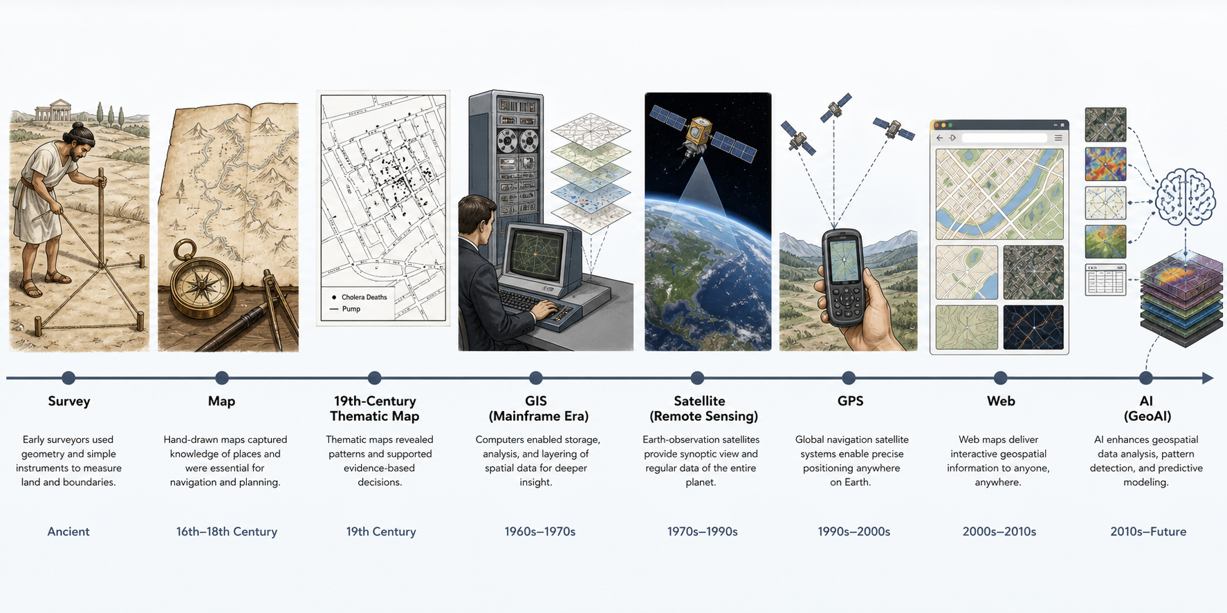
Generated illustration: A conceptual timeline of geospatial technology from ancient surveying and paper maps through GIS, satellites, GPS, web maps, and GeoAI.

Learning Goals

By the end of this chapter, a non-spatial software engineer should be able to:

• Explain why geospatial software emerged from older traditions in surveying, cartography, navigation, astronomy, statistics, and computing.
• Recognize the difference between a map as a visual artifact and a geospatial information system as a data, analysis, and decision platform.
• Describe how coordinate systems, measurement, thematic layers, remote sensing, and databases became core geospatial software ideas.
• Connect early historical examples to modern engineering concerns such as data modeling, indexing, interoperability, uncertainty, and reproducibility.
• Identify major milestones that shaped modern GIS, Earth observation, GPS, web mapping, open standards, and GeoAI.

1.1 Why Location Became a Computing Problem

Location became a computing problem because human decisions have always depended on spatial relationships: where land begins and ends, where water flows, where people live, where disease spreads, where resources exist, and how goods or armies move. Long before digital computers, societies built information systems around place. Cadastral maps recorded land ownership. Nautical charts supported travel and trade. Astronomical tables helped navigators estimate position. Census maps revealed population patterns. Military maps coordinated movement and logistics.

For software engineers, the important shift is this: geospatial technology did not begin as "maps on screens." It began as structured reasoning about position, distance, adjacency, direction, scale, and change. Modern geospatial software simply makes those forms of reasoning programmable.

In ordinary software, a record might answer, "Who is this customer?" or "What is this transaction?" In geospatial software, the record also answers, "Where is it?", "What is near it?", "What contains it?", "What path connects it?", "What changed here?", and "At what scale does the answer remain true?"

1.2 Ancient Mapping, Navigation, Surveying, and Spatial Recordkeeping

Early geospatial practice mixed measurement, representation, law, and survival. Surveying helped establish property, taxation, irrigation, and construction. Navigation supported movement across land and sea. Mapping encoded local and imperial knowledge into portable visual forms.

The ancient engineer did not have GIS, but did have recognizable geospatial concerns:

• Reference points: landmarks, stars, roads, temples, rivers, boundary stones.
• Measurement: distance, bearing, elevation, area, and angle.
• Abstraction: reducing terrain into symbols, lines, labels, and regions.
• Authority: deciding which measurements were trusted enough for law, taxation, or navigation.
• Update cycles: revising records after floods, wars, construction, or settlement change.

These concerns still appear in software. A modern parcel fabric, routing graph, or satellite data cube is a descendant of older practices for turning place into durable information.

Theory

The foundational theory is that spatial information is a model of the world, not the world itself. Every map, dataset, coordinate system, and geospatial API is a selective representation.

Important representational choices include:

• What features are included or excluded.
• Whether features are represented as points, lines, polygons, grids, networks, or fields.
• How uncertainty is recorded.
• Which coordinate system anchors the data.
• Which scale the representation is valid for.

Math

Early spatial math centered on geometry and measurement:

• Distance: how far apart two locations are.
• Angle: how directions relate.
• Area: how much surface is enclosed.
• Proportion: how map distance relates to ground distance.
• Triangulation: how unknown positions can be inferred from known baselines and angles.

For engineers, triangulation is worth remembering because it anticipates later positioning systems. GPS and other GNSS systems use more advanced timing and orbital models, but the engineering instinct is similar: infer a position from relationships to known references.

Tools of the Trade

Historical tools:

• Measuring ropes and chains.
• Groma, diopter, compass, sextant, astrolabe, plane table, and theodolite.
• Paper maps, nautical charts, gazetteers, cadastral records, and survey notebooks.

Modern descendants:

• Total stations, GNSS receivers, drones, mobile mapping systems, GIS databases, and coordinate transformation libraries.

Examples of Real-World Solutions

• Boundary surveys for taxation and land tenure.
• Nautical charts for maritime trade.
• Irrigation and flood-control planning.
• Road and military route planning.
• Early public health mapping.

Working Practice Examples

1. Choose a familiar place such as a campus, neighborhood, or office park. Sketch it as a paper map, then list which features you omitted. Explain how those omissions would affect a navigation app, delivery app, or emergency response app.
2. Measure a simple area manually using approximate dimensions, then compare the result with a polygon drawn in a web map. Identify at least three possible sources of disagreement.
3. Create a small table with name, type, latitude, and longitude columns for ten landmarks. Explain what additional fields would be needed before this becomes production-quality spatial data.

1.3 Astronomy, Geodesy, and the Measurement of Earth

Cartography became more scientific as astronomy, mathematics, and geodesy improved. To map Earth, people needed to know Earth's size and shape, determine latitude and longitude, and translate a curved surface onto flat media.

Claudius Ptolemy's Geography became one of the most influential early works because it joined place descriptions with a coordinate framework. Later mapmakers and geodesists refined these ideas through better instruments, observations, and mathematical models.

Geodesy matters to software engineers because Earth is not a flat Cartesian plane. Coordinates are not just numbers; they are numbers inside a reference system. A latitude-longitude pair without a datum, axis convention, and coordinate reference system is incomplete engineering data.

Theory

Geodesy is the science of measuring and representing Earth. It gives geospatial software a way to connect abstract coordinates to physical locations.

Core ideas:

• Earth can be approximated as a sphere, ellipsoid, or geoid depending on the task.
• Latitude and longitude describe angular position.
• Datums define how a coordinate model is anchored to Earth.
• Map projections transform curved-surface coordinates into planar coordinates.
• Every projection distorts something: area, shape, distance, direction, or scale.

Math

Key mathematical concepts:

• Spherical geometry.
• Ellipsoidal geometry.
• Trigonometry.
• Coordinate transformations.
• Projection equations.
• Error propagation from measurement to mapped output.

For a first mental model, remember that longitude lines converge toward the poles. One degree of longitude is not a constant ground distance everywhere on Earth. Code that treats latitude and longitude as simple x/y coordinates will eventually produce wrong distances, wrong areas, or wrong buffers.

Tools of the Trade

Historical tools:

• Astronomical observations.
• Marine chronometers.
• Sextants and almanacs.
• Survey baselines and triangulation networks.

Modern descendants:

• PROJ, EPSG registry, pyproj, GDAL, PostGIS coordinate operations, GNSS correction services, and geodetic control networks.

Examples of Real-World Solutions

• National mapping programs.
• Maritime navigation.
• Boundary treaties.
• Engineering control networks.
• Satellite positioning and coordinate transformations.

Working Practice Examples

1. Take two points one degree of longitude apart near the equator and two points one degree of longitude apart near 60 degrees north. Calculate or look up their approximate ground distances. Explain why they differ.
2. Find the EPSG code for WGS 84 and a local projected CRS for your region. Write down when each one is appropriate.
3. Use a GIS tool or spatial library to reproject one point from WGS 84 to a projected CRS, then back again. Record any tiny numeric differences and explain why exact round-tripping is not always guaranteed.

1.4 Colonial Mapping, Cadastral Systems, and the Politics of Maps

Maps have never been neutral containers of facts. They have been used to govern, claim, tax, divide, defend, settle, extract, and persuade. Colonial mapping, cadastral systems, and land surveys turned territory into administrative data. These practices helped states and companies manage land, but they also erased or subordinated local, Indigenous, and informal spatial knowledge.

For modern geospatial engineers, this history is not decorative background. It affects data quality, ethics, licensing, trust, and harm. A parcel dataset may encode legal authority. A boundary dataset may encode conflict. A basemap may make some communities visible and others invisible.

Theory

The key theory is that geospatial data has social lineage. A dataset is produced by people and institutions, using categories and measurement methods that reflect goals and power.

Questions engineers should ask:

• Who created the data?
• For what purpose?
• Who was excluded from the data model?
• What legal or political authority does the dataset claim?
• What harms could follow if the dataset is treated as complete or objective?

Math

Relevant mathematical concerns:

• Boundary area calculations.
• Survey closure error.
• Scale-dependent generalization.
• Positional accuracy thresholds.
• Topological consistency between neighboring parcels or administrative regions.

Tools of the Trade

Historical tools:

• Cadastral maps.
• Land ledgers.
• Survey plats.
• Boundary markers.

Modern descendants:

• Parcel fabrics, land administration systems, topology validation tools, versioned geodatabases, and audit trails.

Examples of Real-World Solutions

• Property taxation systems.
• Land titling systems.
• Utility easement management.
• Zoning and permitting platforms.
• Disaster recovery property assessment.

Working Practice Examples

1. Download or inspect a local parcel dataset. Identify its geometry type, key attributes, update frequency, and licensing terms.
2. Look for slivers, gaps, overlaps, or invalid polygons in a parcel or boundary dataset. Explain why these defects matter in legal or operational workflows.
3. Write a short data lineage note for a boundary dataset: source, date, authority, known limitations, and appropriate uses.

1.5 Military Cartography and Early Remote Observation

Military needs accelerated mapping, surveying, aerial photography, satellite reconnaissance, navigation, and later digital geospatial intelligence. Conflict demanded maps that were timely, accurate, portable, and standardized. These requirements shaped modern ideas of coordinate grids, imagery interpretation, terrain analysis, and location-based command systems.

Remote observation also changed the meaning of mapping. Instead of only surveying from the ground, analysts could infer land cover, infrastructure, movement, and change from above. This is one of the roots of remote sensing and Earth observation.

Theory

Military cartography emphasized:

• Standardization across teams and regions.
• Coordinate grids for unambiguous communication.
• Terrain as operational constraint.
• Temporal currency of data.
• Sensor interpretation and uncertainty.

Math

Relevant math includes:

• Line of sight.
• Elevation and slope.
• Photogrammetry.
• Coordinate grids.
• Error ellipses.
• Image registration.

Tools of the Trade

Historical tools:

• Topographic maps.
• Aerial photographs.
• Stereoscopes.
• Grid references.

Modern descendants:

• Digital elevation models, image orthorectification, satellite imagery platforms, SAR, LiDAR, geospatial intelligence systems, and secure tile services.

Examples of Real-World Solutions

• Terrain suitability analysis.
• Infrastructure mapping.
• Change detection.
• Search and rescue.
• Disaster response damage assessment.

Working Practice Examples

1. Compare a satellite image and a vector street map of the same area. List what each one shows better.
2. Use a digital elevation model to calculate slope. Explain how slope might affect wildfire response, road design, or hiking route difficulty.
3. Find two images of the same place from different dates. Identify visible changes and describe how you would automate the comparison.

1.6 Paper Maps, Atlases, Gazetteers, and Coordinate Grids

Before digital GIS, spatial knowledge was distributed through paper maps, atlases, gazetteers, and grid systems. These artifacts remain conceptually important because many modern geospatial data structures preserve their logic.

A gazetteer is a place-name index. A coordinate grid is an addressing system. An atlas is a curated collection of spatial views. A map sheet is a tiled representation of a larger world. These ideas reappear in search indexes, tile pyramids, spatial catalogs, and web map services.

Theory

Paper map systems introduced several enduring concepts:

• Scale controls detail.
• Symbols encode feature classes.
• Indexes support discovery.
• Map sheets partition space.
• Coordinate grids support addressing.
• Legends define semantic meaning.

Math

Relevant math includes:

• Scale ratios.
• Grid indexing.
• Coordinate conversion.
• Generalization thresholds.
• Sheet tiling schemes.

Tools of the Trade

Historical tools:

• Atlases.
• Topographic sheets.
• Gazetteers.
• Map indexes.

Modern descendants:

• Web map tile grids, geocoders, place databases, spatial catalogs, STAC catalogs, and vector tile schemas.

Examples of Real-World Solutions

• Place search.
• Map tile serving.
• Offline field maps.
• National topographic map series.
• Emergency map books and grids.

Working Practice Examples

1. Pick a paper or online topographic map and identify its scale, contour interval, legend, grid, and publication date.
2. Design a tiny gazetteer schema for place names. Include support for alternate names and ambiguous names.
3. Explain how a paper map sheet index resembles a web tile pyramid.

1.7 Early Computers, Mainframes, and the Birth of Digital Mapping

Digital mapping emerged when organizations began using computers to store, process, and analyze map information. Early systems were constrained by expensive hardware, limited storage, batch processing, and specialized input devices. Yet they introduced the central shift from map-as-picture to map-as-data.

Waldo Tobler's 1959 article "Automation and Cartography" anticipated automated map production and computational treatment of geographic information. In the 1960s, the Canada Geographic Information System (CGIS), associated with Roger Tomlinson and the Canada Land Inventory, became a landmark in computerized GIS. Its importance was not merely that maps entered a computer; it was that spatial layers could be stored, combined, queried, and analyzed.

Theory

The birth of digital mapping introduced a new engineering model:

• Spatial features can be encoded as data.
• Layers can represent different themes.
• Attributes can be linked to geometry.
• Spatial operations can be automated.
• Output maps can be generated from underlying data.

Math

Relevant math includes:

• Coordinate encoding.
• Digitization error.
• Polygon overlay.
• Raster grid analysis.
• Boolean logic for suitability analysis.
• Area-weighted aggregation.

Tools of the Trade

Historical tools:

• Mainframes.
• Digitizing tables.
• Line printers.
• Magnetic tape.
• Early plotters.

Modern descendants:

• Desktop GIS, spatial databases, cloud object stores, distributed processing engines, and notebook-based geospatial workflows.

Examples of Real-World Solutions

• Land inventory.
• Resource planning.
• Suitability analysis.
• Thematic mapping.
• Environmental assessment.

Working Practice Examples

1. Create three simple layers: roads, parcels, and flood zones. Perform a spatial overlay to identify parcels touching flood zones and roads.
2. Convert a small vector polygon layer to raster. Explain what information is lost or changed.
3. Write pseudocode for a suitability analysis that scores land based on slope, distance to roads, and distance from wetlands.

1.8 The Canada Geographic Information System and Early GIS

CGIS is widely treated as one of the first operational computerized GIS efforts. It served the Canada Land Inventory, which needed to manage large volumes of land capability data. The system helped formalize ideas that remain central today: spatial layers, attributes, data capture, map overlay, and analysis.

The lesson for software engineers is that GIS was born from a data integration problem. The goal was not to make a prettier map; it was to support decisions that required multiple spatial datasets to be combined consistently.

Theory

Early GIS established the layer model:

• Each layer represents a theme.
• Each feature has geometry and attributes.
• Overlay combines layers to answer compound spatial questions.
• Spatial data quality affects analytical results.
• Data management is as important as visualization.

Math

Relevant math includes:

• Polygon overlay operations.
• Area calculation.
• Reclassification.
• Weighted scoring.
• Topological consistency.

Tools of the Trade

Historical tools:

• CGIS.
• Early land inventory classification systems.
• Digitization workflows.

Modern descendants:

• ArcGIS, QGIS, GRASS GIS, PostGIS, GeoPandas, rasterio, xarray, and cloud-native geospatial processing stacks.

Examples of Real-World Solutions

• Agricultural suitability.
• Forestry inventory.
• Regional planning.
• Soil and land capability mapping.
• Conservation planning.

Working Practice Examples

1. Build a two-layer overlay example with land use and soil class. Identify combinations suitable for a selected use case.
2. Compare a layer-based GIS workflow with a relational database join. Explain what spatial overlay adds beyond attribute joins.
3. Create a simple data dictionary for a land capability dataset.

1.9 Satellite Navigation, GPS, GLONASS, Galileo, and BeiDou

Global Navigation Satellite Systems changed location from a specialized surveying output into a ubiquitous software input. GPS began as a U.S. military system and became a global utility for civilian navigation, logistics, timing, mapping, and mobile computing. Other constellations, including GLONASS, Galileo, and BeiDou, expanded global positioning resilience and availability.

For software engineers, GNSS matters because many systems now assume a device can produce coordinates continuously. But those coordinates are measurements with uncertainty, not perfect facts.

Theory

GNSS positioning relies on signals from satellites with known orbits and highly precise timing. A receiver estimates its position from signal travel times. Accuracy depends on satellite geometry, atmospheric effects, multipath, receiver quality, correction services, and environment.

Math

Relevant math includes:

• Trilateration.
• Time-of-flight measurement.
• Least-squares estimation.
• Error propagation.
• Coordinate reference systems.
• Dilution of precision.

Tools of the Trade

Modern tools:

• GNSS receivers.
• Mobile device location APIs.
• Differential GPS and RTK.
• NMEA streams.
• Positioning SDKs.
• Spatial databases for track storage.

Examples of Real-World Solutions

• Turn-by-turn navigation.
• Fleet tracking.
• Asset management.
• Emergency dispatch.
• Precision agriculture.
• Field data collection.

Working Practice Examples

1. Record a short GPS track on a mobile device. Plot it on a map and identify noise, jumps, or drift.
2. Store a track as timestamped points. Calculate speed between consecutive points and flag impossible values.
3. Compare raw GPS points with snapped-to-road locations. Explain when map matching is helpful and when it can hide reality.

1.10 Landsat, Earth Observation, and Remote Sensing at Scale

Landsat 1 launched on July 23, 1972, as the Earth Resources Technology Satellite. The NASA and USGS Landsat program became the longest continuous space-based record of Earth's land surface, supporting decades of environmental monitoring, agriculture, forestry, geology, urban analysis, and climate research.

This matters because Earth observation turned the planet into a repeatable data product. Instead of only mapping what people surveyed, engineers and scientists could analyze calibrated imagery collected on a schedule.

Theory

Remote sensing measures reflected or emitted energy. Different surfaces interact with different wavelengths in distinctive ways. A satellite image is not just a picture; it is a set of measurements across space, spectrum, and time.

Math

Relevant math includes:

• Raster grids.
• Spectral bands.
• Radiometric calibration.
• Image classification.
• Change detection.
• Time-series analysis.
• Resampling and reprojection.

Tools of the Trade

Modern tools:

• Landsat and Sentinel archives.
• Cloud-Optimized GeoTIFF.
• STAC.
• Google Earth Engine.
• Microsoft Planetary Computer.
• NASA Earthdata.
• rasterio, xarray, rioxarray, GDAL, and Dask.

Examples of Real-World Solutions

• Deforestation monitoring.
• Burn severity mapping.
• Crop health analysis.
• Urban growth detection.
• Water extent monitoring.
• Glacier retreat measurement.

Working Practice Examples

1. Download or access two Landsat scenes for the same area in different years. Compare visible land-cover change.
2. Calculate NDVI from red and near-infrared bands. Explain what high and low values may indicate.
3. Write a processing checklist for turning raw imagery into an analysis-ready dataset.

1.11 Desktop GIS and the Rise of Commercial Geospatial Software

As computing became cheaper and graphical interfaces improved, GIS moved from specialized mainframe environments into desktop software. Commercial vendors and open source projects made spatial analysis available to planners, scientists, engineers, governments, and businesses.

Desktop GIS established workflows that still influence cloud systems: load layers, inspect attributes, style maps, run geoprocessing tools, export results, and share maps.

Theory

Desktop GIS popularized:

• Interactive spatial analysis.
• Visual layer management.
• Geoprocessing workflows.
• Attribute editing.
• Cartographic styling.
• Project files as workflow containers.

Math

Relevant math includes:

• Buffering.
• Intersection.
• Union.
• Dissolve.
• Spatial joins.
• Raster algebra.
• Network routing.

Tools of the Trade

Tools:

• ArcGIS.
• QGIS.
• GRASS GIS.
• MapInfo.
• ERDAS Imagine.
• ENVI.
• GDAL/OGR.

Examples of Real-World Solutions

• Local government planning.
• Environmental impact assessment.
• Utility asset management.
• Business site selection.
• Emergency preparedness.

Working Practice Examples

1. Install QGIS and load a public boundary dataset and road dataset.
2. Perform a buffer around roads, intersect it with parcels, and export the result.
3. Repeat the same operation in SQL or Python and compare the workflow with desktop GIS.

1.12 Open Geospatial Standards and the Open Source GIS Movement

As geospatial systems multiplied, interoperability became a major engineering problem. Different vendors, agencies, and applications needed to exchange spatial data and services. The Open Geospatial Consortium, founded in 1994, became a central institution for open geospatial standards. Standards such as WMS, WFS, WCS, GeoPackage, and newer OGC API standards help systems communicate.

Open source GIS also changed the field. Tools such as GRASS GIS, GDAL, PostGIS, QGIS, PROJ, GEOS, MapServer, GeoServer, and many Python and JavaScript libraries made geospatial software more transparent, extensible, and reproducible.

Theory

Interoperability means that independent systems can exchange and correctly interpret spatial information. In geospatial software, this requires agreement about:

• Geometry models.
• Coordinate reference systems.
• File formats.
• Service protocols.
• Metadata.
• Semantics.
• Error handling.

Math

Relevant math is embedded inside common libraries:

• Coordinate transformations in PROJ.
• Geometry predicates in GEOS.
• Spatial indexing in databases.
• Raster resampling in GDAL.
• Tiling schemes in web maps.

Tools of the Trade

Tools and standards:

• OGC standards.
• GDAL/OGR.
• PROJ.
• GEOS.
• PostGIS.
• QGIS.
• GeoServer.
• MapServer.
• GeoJSON.
• GeoPackage.
• Cloud-Optimized GeoTIFF.
• STAC.
• GeoParquet.

Examples of Real-World Solutions

• Publishing public map services.
• Exchanging data between agencies.
• Building reproducible research workflows.
• Migrating from proprietary-only workflows to hybrid stacks.
• Serving cloud-native imagery and vector data.

Working Practice Examples

1. Convert a GeoJSON file to GeoPackage using GDAL.
2. Publish a local layer through a simple web map service or API.
3. Load the same dataset into QGIS, PostGIS, and a Python notebook. Compare how each tool represents geometry and CRS metadata.

1.13 Lessons from History for Modern Geospatial Engineers

The history of geospatial technology gives software engineers several durable lessons:

1. Spatial data is modeled, not merely collected.
2. Coordinates only make sense inside reference systems.
3. Scale changes meaning.
4. Uncertainty is normal and must be represented.
5. Maps are analytical and political artifacts.
6. Interoperability is a core engineering requirement.
7. The hardest geospatial problems often combine data quality, math, systems design, and institutional context.
8. Modern GeoAI and GeoRAG systems inherit all of these issues rather than replacing them.

In 2026, geospatial software engineering spans databases, APIs, cloud storage, Earth observation, machine learning, streaming systems, digital twins, and AI assistants. But the old questions remain: What is the location? How was it measured? What does it mean? What is near it? What changed? Can the result be trusted?

Theory

History teaches that geospatial engineering is an integration discipline. It combines:

• Measurement science.
• Data modeling.
• Computation.
• Visualization.
• Decision support.
• Governance.
• Ethics.

Math

The recurring mathematical foundation includes:

• Geometry.
• Trigonometry.
• Graph theory.
• Statistics.
• Linear algebra.
• Optimization.
• Signal processing.
• Numerical methods.

Tools of the Trade

Modern geospatial engineers should become comfortable with:

• QGIS for inspection and analysis.
• PostGIS for spatial databases.
• GDAL/OGR for data conversion and processing.
• PROJ for coordinate operations.
• Python geospatial libraries such as GeoPandas, Shapely, rasterio, pyproj, and xarray.
• JavaScript web mapping libraries.
• Cloud object storage.
• STAC catalogs.
• Containerized and reproducible workflows.
• AI-assisted coding and retrieval tools, used with careful source validation.

Examples of Real-World Solutions

• A city uses parcels, zoning, flood zones, and infrastructure layers to evaluate development permits.
• A humanitarian team combines satellite imagery, road networks, and field reports after a disaster.
• A logistics platform combines GPS traces, traffic, routing graphs, and geocoding.
• A climate analytics platform uses decades of Landsat observations to identify land-cover change.
• A GeoRAG assistant retrieves place-specific policy documents, hazard maps, and infrastructure records, then grounds its answer in spatial context.

Working Practice Examples

1. Build a one-page timeline connecting at least ten historical milestones to modern software concepts.
2. Choose one modern geospatial product and identify its historical ancestors: surveying, cartography, remote sensing, spatial statistics, databases, or navigation.
3. Write a short architecture note for a simple geospatial app. Include data sources, coordinate systems, storage, analysis, visualization, and uncertainty.

Chapter 1 Review Questions

1. Why is a map not the same thing as a geospatial information system?
2. What problems arise when latitude and longitude are treated as ordinary Cartesian coordinates?
3. Why did thematic layers become such an important idea in GIS?
4. How did remote sensing change the scale and frequency of spatial data collection?
5. What ethical risks follow from treating historical boundary datasets as neutral facts?
6. Why are open standards especially important in geospatial software?
7. How do modern GeoAI and GeoRAG systems inherit older geospatial data problems?

Image Generation Notes

The chapter illustration was generated for this book using the following prompt:

Create a polished educational illustration showing the evolution of geospatial technology from ancient surveying and paper maps to computer GIS, satellites, GPS, web maps, and GeoAI. Use a clean light-background horizontal timeline suitable for a technical textbook. Show conceptual vignettes for ancient survey, hand-drawn map, disease dot map, mainframe GIS layers, Earth-observation satellite, GPS, web map tiles, and AI-assisted geospatial analysis. Avoid copyrighted map reproductions, logos, brand names, and decorative clutter.

Works Cited

Couclelis, Helen. "Climbing on a Milestone for a Better View: Goodchild's 'Geographical Information Science' Paper as Vantage Point and Ground for Reflection." International Journal of Geographical Information Science, vol. 26, no. 12, 2012, pp. 2291-2300. Taylor & Francis Online, https://doi.org/10.1080/13658816.2012.713959. Accessed 9 May 2026.

Dana, Peter H. "Global Positioning System Overview." The Geographer's Craft Project, University of Colorado Boulder, 1995, https://colorado.edu/geography/gcraft/notes/gps/gps_f.html. Accessed 9 May 2026.

Goodchild, Michael F. "Geographical Information Science." International Journal of Geographical Information Systems, vol. 6, no. 1, 1992, pp. 31-45. Taylor & Francis Online, https://doi.org/10.1080/02693799208901893. Accessed 9 May 2026.

"GPS.gov: GPS Overview." GPS.gov, National Coordination Office for Space-Based Positioning, Navigation, and Timing, https://www.gps.gov/systems/gps/. Accessed 9 May 2026.

"History." Landsat Science, NASA Goddard Space Flight Center, https://landsat.gsfc.nasa.gov/satellites/history/. Accessed 9 May 2026.

"Landsat." NASA Science, National Aeronautics and Space Administration, https://science.nasa.gov/mission/landsat/. Accessed 9 May 2026.

"Landsat 1." NASA Science, National Aeronautics and Space Administration, https://science.nasa.gov/mission/landsat/landsat-1/. Accessed 9 May 2026.

McHarg, Ian L. Design with Nature. Natural History Press, 1969.

Minard, Charles Joseph. Carte Figurative des Pertes Successives en Hommes de l'Armee Francaise dans la Campagne de Russie 1812-1813. 1869. Wikimedia Commons, https://commons.wikimedia.org/wiki/File:Minard.png. Accessed 9 May 2026.

"About OGC." Open Geospatial Consortium, https://www.ogc.org/about/overview/. Accessed 9 May 2026.

Ptolemy, Claudius. Geography. Translated and edited by J. Lennart Berggren and Alexander Jones, Princeton UP, 2000.

Snow, John. On the Mode of Communication of Cholera. 2nd ed., John Churchill, 1855. Lehigh Library Exhibits, https://exhibits.lib.lehigh.edu/exhibits/show/data_visualization/item/3224. Accessed 9 May 2026.

Tobler, Waldo R. "Automation and Cartography." Geographical Review, vol. 49, no. 4, 1959, pp. 526-534.

Tomlinson, Roger F. Thinking about GIS: Geographic Information System Planning for Managers. ESRI Press, 2003.

"Roger Tomlinson, Geographer." Esri, https://www.esri.com/about/newsroom/insider/roger-tomlinson-geographer/. Accessed 9 May 2026.

---